
Point density is the first parameter of an aerial LiDAR survey and the most often misunderstood. It is regularly confused with precision, which it is distinct from, and it is chosen without considering its effect on processing cost.
This article sets out what density determines, what it does not, and how to choose it. It extends the article on the cost of classification.
Density and precision, two distinct notions
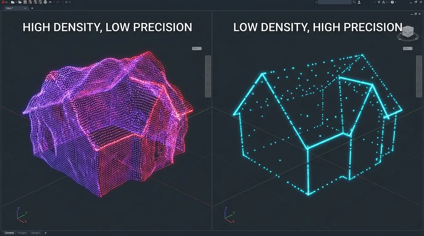
This confusion dominates aerial LiDAR specifications. It deserves clearing before any discussion. Density measures how many points are measured per unit area. It determines what is resolvable, meaning which objects are sampled well enough to be distinguished. Precision measures the discrepancy between a point’s position and the real position of the surface it describes. It determines the correctness of each individual measurement. Three consequences follow. A survey can be dense and imprecise, where the positioning system is defective, each point being measured frequently and badly placed. A survey can be precise and sparse, each point being exactly positioned while thin objects escape sampling. And the two are specified separately, a specification stating a density without an accuracy describing only half the expected product.What aerial LiDAR density determines
Four properties of a survey depend on it directly. The size of the smallest detectable object, an empirical rule holding that an object must receive several pulses to be reliably identified. The fineness of the terrain model, the useful grid resolution being bounded by the mean spacing between ground points as the corresponding article established. Effective penetration under canopy, a higher density mechanically increasing the number of pulses reaching the ground through gaps in the foliage. And classification reliability, an object described by many points presenting an identifiable geometry that one described by three points does not. One important observation follows. That fourth property is the most neglected at scoping, density being discussed in terms of visible detail when it also conditions the feasibility of annotation.What density does not determine
Four limits rule out unrealistic expectations. Vertical accuracy depends on the positioning system and the calibration, not on the number of points. Classification quality depends on the method and the human work, a high density easing the work without doing it. Surface nature escapes this modality entirely, more points not producing colour information. And penetration under very dense canopy stays bounded, a higher density increasing the number of ground points in zones where some pulses pass and creating none where none pass. That last limit is the most often ignored. Under a closed canopy in full leaf, raising the density does not solve the problem, where changing season does.Nominal density and real density
This distinction explains discrepancies observed in aerial LiDAR production. The density stated in a specification is a mean value across a whole survey. Four factors make it vary locally. Overlap between flight strips, overlap zones presenting double density. The nature of the surface, an absorbing or reflecting surface returning fewer usable echoes. The incidence angle, swath edges presenting lower density and more spread footprints. And vegetation cover, which intercepts a share of the pulses before they reach the ground. One practical consequence follows for an aerial LiDAR project. Ground point density, the only relevant one for a terrain model, is far below total density in wooded areas, and it is that value that must be checked rather than the nominal one.The components of precision
This decomposition permits attributing a defect to its cause. Five error sources combine in a point’s position. The distance measurement itself, generally the smallest of the five, laser metrology being mature. The aircraft’s position, whose quality depends on the satellite receiver and the trajectory processing. Orientation, measured by the inertial unit, where an angular error produces a displacement growing with distance from the sensor. System calibration, the alignment between sensor and inertial unit, whose defect produces a systematic error. And the nature of the surface, a steep slope or a diffusing surface spreading the footprint and making the position less defined. One important observation follows for an aerial LiDAR project. Vertical precision is generally better than horizontal precision, the angular error affecting mainly the planimetric component, which explains why specifications distinguish the two and why altimetric uses are the most reliable.The relationship between density and cost
This economic relationship plays on both sides. It governs this choice. On acquisition, density is obtained by flying lower or slower, which reduces the area covered per flight hour and raises the cost per unit area. On processing, density increases the data volume, therefore the storage, the computation time and the annotation time. Three observations follow. Cost grows on both lines simultaneously, which makes the relationship between density and total cost more than proportional. Density is therefore the most decisive budget parameter after area, and its choice deserves an examination most projects do not give it. And a density above the need is not recoverable, the data being acquired and the processing cost applying to each point whether wanted or not. One qualification nonetheless deserves making. Downsampling is possible at processing, which permits acquiring dense and processing light where several uses coexist, at the price of storage.Densities by use
An indicative correspondence helps at scoping, subject to landscape and season modifying it. A terrain model over wide extents makes do with a modest density, a few points per square metre sufficing in open terrain. Building mapping requires more, a roof’s form presupposing enough points to fit its pitches. Plot-based forest inventory requires an intermediate density, statistical metrics tolerating moderate sampling. Individual tree detection requires a high density, crowns needing to be separable. And network corridor management requires the highest density, detecting thin cables imposing several pulses per object. One observation runs across that correspondence. The gap between the first and the last use is measured in an order of magnitude, which explains why the same territory is flown several times for different needs rather than once at maximum density.How to choose a density
Four questions determine the value needed. They are asked in one meeting. What is the smallest object to identify. That answer sets a floor, the object having to receive several pulses. Is ground under canopy needed. A positive answer requires reasoning on ground point density rather than total density, a considerable gap in wooded areas. What model resolution is expected. That answer translates directly into the mean spacing required. And what area is concerned. That answer determines whether a high density is economically sustainable. One observation follows. Those four answers produce a value rather than a range, and that value is almost always below what a project would have adopted out of caution.The question of homogeneity
One property matters more than the mean value for most uses and it is rarely specified. A survey of homogeneous density and one of the same mean density but highly variable do not permit the same things. Three reasons explain that. The least dense zones bound what the product can guarantee, a model being reliable only where the points exist. Variability complicates parameterisation, a classification setting suited to dense zones failing on sparse ones. And it precludes a single resolution, the useful grid differing from one sector to another. One practical consequence follows. Specifying a minimum value per unit area rather than a global mean protects the use, and that formulation costs the client little while genuinely committing the supplier.Verifying the density of a survey received
This operation establishes what an aerial LiDAR survey actually permits. It takes minutes. Four measurements compose that verification. Total density per unit area, computed over several contrasting sectors rather than as a global mean. The density of points classified as ground, the only relevant one for a terrain model, to be compared against the previous one in wooded areas. The density map, a representation showing the spatial distribution and revealing overlap strips as well as sparse zones. And the mean spacing between ground points, a value translating directly into useful grid resolution. One practical consequence follows. Those four measurements reveal in minutes that a survey stated at a given density does not present it everywhere, information that changes what a project can promise and that appears in no metadata. One observation completes that. Delivering a density map alongside a model is the most useful and cheapest complement an aerial LiDAR provider can offer, and almost nobody proposes it.Strip adjustment
One operation conditions a survey’s consistency and its defect produces a recognisable signature. Two passes over the same area never coincide exactly, each carrying its own trajectory’s errors. Three manifestations reveal an adjustment defect. Doubled surfaces in the overlap zone, visible in section as two offset parallel planes. Regular undulations in the terrain model, aligned on the flight axes. And elevation discontinuities at strip limits, an object appearing higher on one side than the other. One practical consequence follows for an aerial LiDAR project. This defect belongs to acquisition rather than to classification, it is not corrected by annotation work, and confusing it with a classification error leads to spending effort on a problem that calls for upstream reprocessing. One observation completes that. Checking consistency in the overlap zone before committing to a classification avoids processing data that will have to be redone, a check taking minutes that few projects conduct.Checking precision
Three methods verify the stated accuracy of an aerial LiDAR survey. They combine usefully. Comparison against ground control points surveyed by a geometrician, the only absolute verification and necessarily pointwise, whose sample must cover several surface and slope types. Internal consistency in the overlap zone, measuring the discrepancy between two passes over the same surface and informing about relative precision with no external truth. And comparison against an earlier survey over stable surfaces, carriageways and roofs, whose discrepancy should be nil and whose value measures consistency between campaigns. One important observation follows for a project. The second method costs nothing and it is rarely practised, though a large discrepancy in the overlap zone invalidates any precision claim whatever the comparison against control points. One practical consequence follows. This check is conducted before committing to a classification, a precision defect belonging to acquisition and making any annotation work on data that will be redone pointless.What density changes for annotation
An inverse reading deserves stating because it directly concerns a data provider. Density modifies the nature of annotation work as much as its volume. Four effects are distinguishable. Recognition becomes easier, an object described by many points presenting an identifiable geometry a few points do not show. Interfaces become sharper, the limit between two classes locating with more fineness. The volume to handle grows proportionally, which lengthens every selection and verification operation. And ambiguous cases multiply, a high density revealing configurations low density masked and which require a decision. That fourth effect is counterintuitive and deserves emphasis. A higher density does not uniformly simplify the work, it makes visible difficulties that undersampling concealed, which requires a fuller case library.Downsampling as a tool
This operation resolves several of the difficulties set out above. Deliberately reducing a cloud’s density produces a lighter set whose geometry stays correct. Four uses follow. Rapid exploration of a wide territory, a lightened version displaying fluidly where the full cloud saturates a workstation. Harmonising surveys of differing densities, bringing the denser down to the level of the sparser making two campaigns comparable. Training models, downsampling reducing computation cost without necessarily degrading performance. And delivery to a client whose uses do not require the full density. Three methods are distinguishable and their choice matters. Random draw, simple and degrading spatial regularity. Grid downsampling, preserving a homogeneous distribution and better suited to geometric processing. And retaining only first or last returns, preserving one particular kind of information at the price of the others. One practical consequence follows for an aerial LiDAR project. Downsampling is done at processing and never at acquisition, a density not acquired not being recoverable, which argues for acquiring at the level of the most demanding need where several uses coexist.Expressing a density requirement
An operational formulation is better than a bare value and it is built in three steps. Establish first the smallest object to identify and the position precision expected on that object, two distinct requirements translating separately. State next whether the requirement concerns total density or ground point density, a decisive distinction in wooded areas and rarely made explicit in specifications. And fix finally how conformity will be verified, global mean or minimum value per unit area, those two formulations not committing a supplier equally. One practical consequence follows. A requirement framed this way is verifiable and it protects both parties, where a single nominal value permits delivering a survey conforming on average and insufficient where the project needs it.Five checks before committing to a project
This list condenses the chapter into an aerial LiDAR check applicable quickly. It takes under an hour. Total density measured over several contrasting sectors, rather than the stated value. Ground point density over wooded sectors, the value conditioning the terrain model. Consistency in the overlap zone, revealing an adjustment defect that invalidates any precision claim. The acquisition season, which determines what the ground point density could reach. And the translation of those values into capability, smallest identifiable object and useful model resolution. One observation follows. Those five checks require no particular tooling or rare competence, and their omission explains a share of the projects that discover late that their base data did not support what they expected of it.What this chapter teaches
One cross-cutting observation deserves closing this examination because it holds beyond this parameter. Density is a single figure that poorly describes a variable reality, and that property recurs in most technical specifications. Three findings compose it. The nominal value is a mean, and the mean masks a spatial variation that can reach a factor according to surface and cover. The relevant value depends on the use, total density and ground point density answering different questions. And the figure stated says nothing about what it permits, the translation into identifiable objects and model resolution requiring a reasoning the specification does not perform. One consequence follows for an aerial LiDAR provider. Knowing how to translate a specification into real capability is a scoping competence distinct from production competence, it is exercised in minutes, and it avoids projects committed on data that did not permit what was expected of them.Reading a survey you did not commission
One aerial LiDAR situation recurs and it deserves a sequence, since most projects inherit a survey rather than specify one. The question is not whether the survey is good but whether it supports the intended use, and those are different questions with different answers. Four steps answer it. State the use in terms of the smallest object that must be identified and the position precision required on it. Measure what the survey actually delivers on the sectors that matter, using the four measurements set out above rather than the metadata. Compare the two, which produces one of three outcomes: the survey supports the use, it supports it partially over some sectors, or it does not. And where the answer is partial, map where, since a survey supporting the use over eighty per cent of the area is a different proposition from one that fails uniformly. That fourth step is the one that turns a negative finding into a workable project. A partial answer permits scoping the work to the sectors that hold and commissioning a complement for the rest, where a bare verdict of unsuitable closes the conversation.Common mistakes
These failures recur often enough that naming them is usually enough to avoid them.- Confusing density with precision.
- Specifying a density without specifying an accuracy.
- Reasoning on total density rather than ground point density in wooded areas.
- Raising the density to solve a penetration problem under dense canopy.
- Choosing a model resolution finer than the density permits.
- Neglecting density’s effect on processing and annotation cost.
- Adopting a density out of caution rather than by calculation.
- Ignoring the local variation in density between strips and swath edges.
- Expecting a high density to compensate a mediocre classification.
- Comparing two surveys of differing densities without harmonisation.
- Confusing a strip adjustment defect with a classification error.
- Specifying a mean density without a minimum value per unit area.