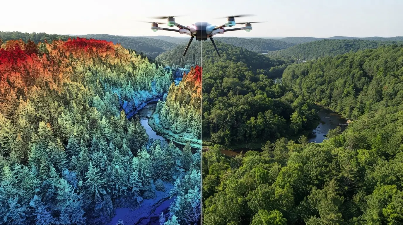
Aerial LiDAR and photogrammetry both produce georeferenced three-dimensional point clouds. That similarity of deliverable masks a difference in kind that determines what each permits.
The first measures distances, the second reconstructs geometry from several images. This article sets out what that difference implies and how to decide between them. It extends the article on
aerial LiDAR.
Two different principles
One founding difference separates these two acquisition techniques and it explains everything that follows.
Aerial LiDAR emits a pulse and measures its return time, which gives a distance directly. The measurement is active and it depends on no interpretation.
Photogrammetry acquires several images of one area from different angles, identifies matching points between them and derives a position by intersection. The measurement is passive and it rests on a correspondence.
Three consequences follow immediately for a project. Photogrammetry requires points to be identifiable across several images, which presupposes texture. It requires illumination, therefore daytime acquisition in clear weather. And it can only measure what is visible from several viewpoints.
Aerial LiDAR meets none of those three constraints, which is its principal advantage.
The question of vegetation cover
One difference dominates this comparison and it settles most decisions.
A laser pulse divides when it meets a vegetation canopy, part passing through and sometimes reaching the ground, a property the opening article detailed.
Photogrammetry cannot reproduce that behaviour. It reconstructs what is visible, meaning the top of the canopy, and the ground under forest escapes it entirely.
Three practical consequences follow directly. A terrain model under forest cover is obtainable only through aerial LiDAR. A surface model is obtainable through both techniques with comparable quality. And a vegetation height measurement requires the former, the difference between surface and terrain presupposing both are known.
That distinction alone settles forestry, hydrology and archaeology projects, where ground under vegetation is the information sought.
The question of texture
An inverse constraint limits photogrammetry and it deserves stating too.
Matching between images requires identifiable patterns. A uniform surface supplies no reference point, which produces a wrong or absent reconstruction.
Four situations defeat it clearly. Water surfaces, whose appearance changes between shots. Uniform surfaces, sand, snow or homogeneous roofing. Shadowed areas, where contrast is insufficient. And reflective surfaces, whose appearance depends on the viewing angle.
Aerial LiDAR meets a difficulty on water, laser absorption producing an absence of return, and it handles the other three without difficulty.
Comparative precision
A technical comparison deserves qualifying here because the two techniques do not degrade in the same way.
In vertical precision, aerial LiDAR is markedly superior. The distance measurement is direct and the error stays stable whatever the conditions.
In horizontal precision, the gap narrows. High resolution photogrammetry reaches comparable precision on textured, well lit surfaces.
In point density, photogrammetry can exceed aerial LiDAR on favourable surfaces, dense matching producing one point per image pixel.
And in homogeneity, aerial LiDAR is superior, its precision varying little with surface nature where photogrammetry’s collapses on untextured surfaces.
One important observation necessarily follows. A comparison on a favourable area, urban and textured, favours photogrammetry; the same comparison on a forested or uniform area inverts the result, which makes any general comparison misleading.
Comparative cost
An economic difference largely explains the persistence of both techniques.
Photogrammetry uses markedly cheaper sensors, a quality camera costing a fraction of a laser scanner.
It requires more overlap between shots in return, therefore more flight lines for the same area, which increases acquisition time.
Photogrammetric processing is heavier in computation, matching and reconstruction requiring substantial resources.
And aerial LiDAR produces a more directly usable deliverable, classification being the only heavy stage where photogrammetry adds reconstruction.
One important practical consequence follows for small footprints. A photogrammetric drone is the cheapest solution over a few hectares, while an aerial LiDAR survey becomes competitive as soon as the area grows or vegetation cover intervenes.
Colour, photogrammetry’s advantage
An advantage specific to the second technique deserves flagging because it weighs in certain uses.
A photogrammetric point natively carries a colour, that of the pixel it came from, which produces a cloud directly interpretable visually.
An aerial LiDAR point carries no colour, only a return intensity whose interpretation is delicate.
Three consequences follow. Photogrammetric annotation is more intuitive, an annotator recognising objects by appearance as much as by form. Producing a textured model is immediate, which matters for visualisation and communication. And identifying surface nature is possible, which geometry alone does not permit.
An answer exists on the aerial LiDAR side and it deserves knowing. Colourising a point cloud with imagery acquired simultaneously combines both advantages, a routine operation an article in this series details.
Operational constraints
Four practical differences separate the two techniques at acquisition and they weigh more than theoretical considerations.
The weather window differs markedly. Photogrammetry requires clear sky and homogeneous illumination, which strongly restricts available slots in cloudy regions. Aerial LiDAR tolerates cloud cover as long as the ceiling stays above flight altitude.
The daily window differs too. Photogrammetry avoids hours of long shadows, which reduces the useful day to a few hours around solar noon. Aerial LiDAR flies indifferently, including at night, which doubles a carrier’s daily capacity.
The overlap constraint weighs on photogrammetry, which requires each point to appear on several images, therefore closely spaced flight lines.
And processing time differs, photogrammetric reconstruction requiring substantial computation where an aerial LiDAR survey is usable soon after georeferencing.
Those four constraints explain part of the real cost. A photogrammetric campaign can wait weeks for a favourable window, an immobilisation the initial quotation does not reflect.
The cases that settle it
Five configurations determine the choice unambiguously and they are worth identifying.
Ground under forest cover imposes aerial LiDAR, photogrammetry not measuring it.
Vegetation height measurement equally imposes aerial LiDAR, for the same reason.
Small footprints without dense vegetation clearly favour drone photogrammetry, whose deployment cost is modest.
Narrow linear features, networks and infrastructure, favour helicopter aerial LiDAR, whose geometric precision and ability to measure thin cables are decisive.
And projects requiring texture, urban modelling for visualisation notably, favour photogrammetry or a combination.
Cables and thin objects
One configuration deserves separate treatment because it separates the two techniques unambiguously.
A power cable, a fence or a thin mast are objects whose cross-section is far below the acquisition resolution.
Aerial LiDAR measures them nonetheless, a pulse meeting the cable producing an echo at the correct distance, independently of the cable occupying only a fraction of the laser footprint.
Photogrammetry fails on these objects. A cable occupies a fraction of a pixel, it produces no correlatable pattern, and the reconstruction ignores it or places it anywhere.
Three consequences follow. Power network management imposes aerial LiDAR, which an article in this series develops. Clearance checking on linear infrastructure equally. And any project concerning thin objects must verify that constraint before deciding on cost.
That configuration illustrates this comparison’s general principle. A physical impossibility settles the matter where a comparison of average precision would suggest equivalence.
Combining the two
One configuration deserves describing because it is often the best answer.
The two techniques combine naturally, their strengths and weaknesses being complementary.
Three different arrangements are used in practice. Simultaneous acquisition, a carrier taking both sensors, which guarantees geometric and temporal coincidence. Colourising an aerial LiDAR cloud with separate imagery, simpler and requiring registration. And sequential use, frequent photogrammetry complementing a reference aerial LiDAR survey acquired more rarely.
That third arrangement particularly deserves emphasis. Aerial LiDAR supplies a precise and expensive reference geometry, photogrammetry supplies frequent and cheap updates, and the combination produces monitoring neither offers alone.
The case of national programmes
One particular configuration deserves flagging because it modifies this decision in several countries.
National aerial LiDAR coverage programmes, which an article in this series details, make freely available data whose acquisition was the principal cost line.
Three consequences follow for this comparison.
Over covered areas, the economic argument for photogrammetry disappears, the aerial LiDAR data being already acquired and paid for.
Photogrammetry retains a freshness advantage, a national survey being several years old where a drone flight is scheduled in days.
And the combination becomes natural, the national survey supplying a reference geometry and an occasional photogrammetric acquisition supplying the update.
One practical consequence follows for a project. Checking national coverage before any decision is the first step, a positive answer radically changing the terms of the comparison.
Terrestrial and mobile LiDAR
A third family deserves situating because it completes the picture and combines with both preceding ones.
Terrestrial LiDAR, static or vehicle-mounted, measures from the ground rather than from the air, which inverts the acquisition geometry.
Three advantages follow. Vertical surfaces are correctly measured, facades and structures notably, where an airborne sensor undersamples them. Density reached is far higher, a terrestrial survey producing thousands of points per square metre. And deployment cost is modest over a small footprint.
Three limits accompany it. Coverage is low, a terrestrial survey covering only what is visible from the roadway or from the stations. Roofs escape this modality entirely. And occlusion is severe in built-up areas, each object masking others.
One practical consequence follows for detailed urban modelling. Aerial LiDAR supplies the roofs and the overall geometry, terrestrial supplies the facades, and their combination produces a complete model neither gives alone.
What this changes for annotation
Four differences distinguish annotating the two types of cloud and they justify separate treatment.
The presence of colour changes the method, a photogrammetric annotator relying on appearance where an aerial LiDAR annotator relies on form.
The noise differs in nature, a photogrammetric cloud carrying correlation artefacts in poorly textured zones and an aerial LiDAR cloud carrying isolated spurious echoes.
Vertical structure exists only in aerial LiDAR, which makes distinguishing vegetation from ground impossible in photogrammetry under canopy.
And density varies differently, a photogrammetric cloud being dense on textured surfaces and sparse elsewhere, where an aerial LiDAR cloud is more homogeneous.
One practical consequence follows. An annotation protocol designed for one technique does not transpose directly to the other, and the conventions at interfaces differ.
Recognising a cloud’s origin
One practical skill deserves setting out because a provider often receives a cloud without its provenance being stated.
Five simple indicators permit deciding in minutes.
The presence of colour on each point generally signals a photogrammetric origin or a colourised aerial LiDAR cloud, which the metadata permits distinguishing.
The presence of echo attributes, number and total count, signals a LiDAR origin unambiguously, photogrammetry not producing that information.
The density distribution also informs, a photogrammetric cloud being dense on textured surfaces and sparse on uniform ones, where an aerial LiDAR cloud is more homogeneous.
The presence of points under vegetation cover settles it definitively, only aerial LiDAR producing them.
And the nature of the noise differs, photogrammetry producing noisy surfaces and correlation artefacts where aerial LiDAR produces isolated spurious points.
One practical consequence follows. Establishing the origin before defining an annotation protocol avoids applying unsuitable conventions, notably on the distinction between ground and low vegetation which does not mean the same thing in both cases.
How to decide in practice
Five questions determine the choice and they are asked in one meeting.
Is ground under vegetation needed. A positive answer imposes aerial LiDAR and closes the discussion.
Is the area concerned small or extensive. Small footprints favour drone photogrammetry, large ones airborne flight.
Are the surfaces to be measured textured. A negative answer, water, sand or uniform roofs, rules out photogrammetry.
Is colour needed in the deliverable. A positive answer points to photogrammetry or to a combination.
And what vertical precision is required. A high requirement favours aerial LiDAR, whose direct measurement is more stable.
What photogrammetry has gained recently
One development deserves flagging because it has narrowed the gap on several points.
Three notable advances have improved this technique over the past decade.
Dense matching algorithms now produce one point per pixel rather than sparse points, which has considerably increased the density obtained on textured surfaces.
Drones have lowered acquisition cost on small footprints, making accessible a technique that previously required an aircraft.
And learned reconstruction improves the handling of weakly textured zones, without lifting the fundamental limit.
Two limits remain unchanged and they are physical rather than technical.
Vegetation penetration remains impossible, no algorithmic advance permitting reconstruction of what is visible on no image.
And measuring thin objects remains defective, a cable not occupying enough pixels to be matched whatever the method.
One practical consequence follows for a decision. Photogrammetry’s advances have shifted the frontier on open surfaces and they have changed nothing on the two configurations where aerial LiDAR is indispensable, which makes this decision more stable than it appears.
Errors of comparison
Four biases regularly distort published comparisons and they are worth knowing.
The favourable test area, a comparison conducted in a textured, well lit urban setting systematically favouring photogrammetry.
Confusing density with precision, a dense photogrammetric cloud potentially being less precise than a sparser aerial LiDAR one.
Omitting vegetation cover, the comparison covering surfaces where both techniques work and ignoring those where one fails.
And comparing costs at unequal scope, a cheap photogrammetric acquisition producing a deliverable requiring more processing.
Those four biases share a common property. All favour photogrammetry, which explains part of the gap between published comparisons and practitioners’ experience.
Framing the recommendation to a client
One commercial observation closes this examination because the comparison lands badly when approached head on.
A client who has already chosen a technique defends it, and a comparison presented as a verdict installs a pointless opposition.
Three framings work better.
Starting from the need rather than the technique, the question of ground under canopy or of thin objects settling itself without an opinion being needed.
Acknowledging what the chosen technique brings, drone photogrammetry genuinely being the best answer over a small open footprint.
And proposing combination rather than substitution, which preserves the investment already made and adds what is missing.
That third framing is the most effective in practice. It turns a challenge into a complement, which is both more accurate technically and better received.
What this comparison teaches
One cross-cutting observation deserves closing this examination because it holds beyond these two techniques.
The question posed is not which is better but which measures what the project is looking for.
Three lessons follow.
A comparison of performance without stating the measurement context informs nothing, the two techniques degrading on opposite configurations.
A physical constraint settles more reliably than an economic trade-off, the impossibility of measuring ground under canopy ruling out a technique whatever its price.
And combination is often better than choice, each one’s weaknesses being the other’s strengths, which explains the frequency of mixed acquisitions.
One practical consequence follows for an annotation provider. Knowing which technique a point cloud came from changes how it is annotated, which makes that question information to obtain at scoping rather than a provenance detail.
What each technique costs to annotate
One observation deserves adding because the comparison usually stops at acquisition and the downstream cost differs too.
Four factors separate the annotation cost of the two cloud types.
Colour helps considerably. A photogrammetric annotator recognises objects by appearance, which shortens training and raises throughput on classes an aerial LiDAR annotator must identify by form alone.
Noise costs differently. Correlation artefacts in untextured zones are dense and structured, which makes them tedious to clean, where isolated spurious LiDAR points are removed by automatic filtering.
Vertical structure changes what is possible. Separating ground from low vegetation is straightforward with echo attributes and largely guesswork without them, which makes some classes far more expensive on photogrammetric data.
And density heterogeneity complicates photogrammetric work, an annotator meeting dense zones and gaps in the same scene without the gap indicating an absence of object.
One conclusion follows. Photogrammetric clouds are cheaper to annotate on simple open scenes and more expensive on vegetated or untextured ones, which mirrors the acquisition comparison rather than offsetting it.
That symmetry is worth noting in a quotation. The technique that is cheaper to acquire in a given context is generally also cheaper to annotate there, which means the total cost gap is wider than the acquisition gap alone suggests.
The decision in one sentence
A closing simplification serves the reader who wants the answer without the reasoning.
If the project needs to know what is under the vegetation, or needs to measure something thinner than a pixel, the answer is aerial LiDAR and no cost argument changes it.
If the project covers a small open area and wants colour, the answer is drone photogrammetry and no precision argument changes it.
Everywhere between those two poles, the decision is genuinely open and it turns on the area, the budget and whether a national survey already exists.
One observation completes that. Most real projects sit at one of the two poles rather than in between, which means the decision is usually clearer than the length of this article suggests. The reasoning matters for the minority of cases where it is not.
What to take away
Both techniques produce a point cloud and they do not measure the same thing, one recording a distance and the other reconstructing geometry from images.
Three readings emerge. Ground under vegetation cover is measurable only through aerial LiDAR, photogrammetry reconstructing only what is visible, which alone settles forestry, hydrology and archaeology projects. Photogrammetry requires texture and illumination, which defeats it on water, uniform surfaces and shadowed areas, where aerial LiDAR keeps a homogeneous precision. And a comparison conducted in a textured urban area systematically favours photogrammetry where the same comparison in a forested area inverts the result, which makes any general comparison misleading.
For the heart of the annotation work, the article on
classifying a point cloud sets out the method. For the general frame, the article on
aerial LiDAR presents this series’ panorama.
To explore delivery arrangements, supported formats and applicable control mechanisms, see our dedicated page on
geospatial data processing. And if you need a point cloud classified, whatever its origin,
let us discuss your project.