
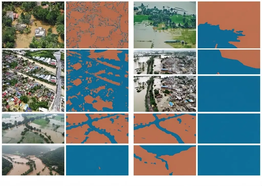
Water is by some distance the easiest class to detect in satellite image segmentation and one of the hardest to map correctly. That apparent paradox rests entirely on a distinction the nomenclature article flagged: a water surface at one date and a flood-prone zone are not the same thing.
This article sets out that distinction, the difficulties specific to this domain and the conventions a project must fix. It extends the article on designing a land cover nomenclature.
Why water is easy to detect
One physical property explains that apparent ease in satellite image segmentation. It also illuminates precisely the cases where it stops working. Water strongly absorbs radiation in the near and mid infrared, where vegetation and soils reflect markedly. A water surface therefore appears very dark in those bands, producing a contrast few other classes present. That physical property gave rise to normalised indices combining a visible band and an infrared one, whose computation is immediate and whose thresholding produces an acceptable first delineation in minutes. Three practical consequences follow directly. A project covering permanent and extensive water bodies obtains a usable result with modest means. Infrared bands are indispensable, imagery limited to the visible performing markedly worse on this class. And performance announced on test sets composed mainly of lakes and rivers substantially overstates what will be obtained on difficult configurations.Where the ease stops in satellite image segmentation
Six configurations defeat the index approach. They constitute the bulk of the real work. Shallow and turbid waters reflect markedly more, through visible bottom and suspended matter, which brings them closer to bare soil. Shadows present a spectral signature close to water in satellite image segmentation, which produces systematic false detections in relief and in dense urban settings. Dark artificial surfaces, some roofs, pavements and panels, produce the same effect. Aquatic vegetation partly masks the water surface, which moves a vegetated water body to the vegetation side. Frozen surfaces completely invert the spectral signature, ice and snow being highly reflective where liquid water is absorbing. And small linear objects, narrow watercourses and irrigation canals, fall below the available resolution or occupy only a fraction of a pixel, which makes them undetectable by thresholding. Those six configurations largely explain the gap between a convincing demonstration and an operational product, and they justify machine learning where a simple index would suffice on easy cases.The founding distinction
This nomenclature decision precedes everything else. Omitting it produces a deliverable that nobody quite knows how to interpret. A water surface observed by satellite image segmentation describes the state at the acquisition date. It is verifiable on the image and it changes from one acquisition to the next. A flood-prone zone describes a property of the territory, defined by a frequency or a probability of inundation. It is not observed on an image but established from a series of observations or from hydraulic modelling. A wetland describes something else again: an environment characterised by soil saturation, adapted vegetation and ecological functioning, whose definition belongs to regulatory references and which does not imply the presence of open water. Those three notions are nonetheless regularly confused, and the confusion produces three kinds of difficulty. A client expecting a flood-prone zone and receiving an observed surface obtains a product unusable for their need. A model trained on labels mixing the three learns an incoherent category. And an evaluation comparing an observed surface against a wetland reference measures a disagreement with no meaning.What each notion requires
The three call for distinct methods in satellite image segmentation. Their cost differs considerably. The observed water surface is produced by segmentation of a single acquisition. That is the simplest and cheapest case. Maximum historical extent is produced by aggregating a series, retaining pixels that were water at least once over the period. It requires a series and a treatment of missing acquisitions. Inundation frequency is produced by counting over the whole series, relating the number of water observations to the number of usable observations. That normalisation is absolutely decisive: a pixel frequently masked by cloud must be treated differently from a pixel frequently dry. And a regulatory flood zone belongs to hydraulic modelling integrating topography, hydrology and structures, to which satellite observation contributes validation rather than production. That last point deserves stating clearly in a commercial discussion. An imagery provider does not produce a regulatory flood zone; it produces observations contributing to establishing or verifying one.Radar and flood mapping
This capability is decisive in the domain’s most operational use. A flood generally occurs under cloud cover, which makes optical imagery inoperative at precisely the moment observation matters. Radar, independent of weather and illumination, removes that constraint. The physical mechanism is particularly favourable there. A calm water surface reflects the radar signal away from the sensor, which makes it appear very dark, with a contrast often exceeding that of optical imagery. Four specific difficulties nonetheless accompany radar. Wind roughens the surface and increases backscatter, which can eliminate the contrast. Smooth non-aqueous surfaces, some roads and tracks, produce the same dark effect. Water under vegetation cover is poorly detected in standard configuration, the canopy masking the surface. And relief produces radar shadow zones also showing a weak signal. One important practical consequence follows for annotation. A flood mapping corpus must be built on radar imagery, with the conventions specific to that modality, and an annotator used to optical work must be trained in a different reading.The satellite image segmentation conventions to fix
Seven distinct decisions must be settled before production begins. Omitting them produces substantial variability. The exact position of the limit on a gentle bank, a sloping shore producing a gradual transition whose exact line is conventional. The treatment of emergent aquatic vegetation, reed beds and beds of aquatic plants, which belongs to water, to vegetation or to a class of its own. The treatment of artificial water surfaces, basins, pools and treatment plants, whose inclusion depends on the purpose. The size threshold below which a water body is not represented, which restates the minimum mapping unit question. The minimum width for a watercourse represented as a surface rather than as a line, a decision that changes the nature of the deliverable. The treatment of ambiguous shadowed areas, which must receive an explicit rule rather than being left to judgement. And the treatment of frozen surfaces, which belong to a distinct class in most nomenclatures and whose omission produces a seasonal discontinuity.Optical and radar fusion in satellite image segmentation
This combined approach addresses the limits of each modality taken alone. The principle is to use both sources over the same area of interest, exploiting their complementary weaknesses. Three configurations benefit particularly. Water under vegetation, poorly seen in standard radar and sometimes discernible optically where the canopy is sparse. Smooth non-aqueous surfaces, dark in radar and distinguishable optically by their spectral signature. And cloudy periods, where radar takes over from an interrupted optical series. Two serious difficulties accompany that combination. Temporal coincidence, two acquisitions of different modalities not being simultaneous, which is a problem on a phenomenon evolving in hours. And geometric coincidence, the two products having to overlay at the required precision, a question the near real-time article raised regarding geolocation. One practical consequence follows for a multimodal project. The corpus must contain annotated examples in both modalities, ideally over the same areas, which doubles the annotation work and constitutes precisely the resource few projects hold.The temporal question
This difficulty dominates this domain more than any other. Water is by far the most variable class over time. The same pixel can be water, dry or intermediate depending on season, year and event, which makes an annotation valid at one date and wrong at another. Three consequences follow directly for building an annotated corpus. The acquisition date must be retained with each annotation, an obvious requirement and regularly omitted. A corpus built over a single season does not allow a product intended to work year-round to be evaluated. And evaluation must cover extreme conditions, low water and flood, which are precisely those where the product will be consulted. A fourth consequence also deserves flagging. A disagreement between an annotation and a reference may arise from a date discrepancy rather than an error, which makes checking dates a prerequisite to any quality diagnosis.Derived products from a water series
A satellite image segmentation series supports several indicators a client regularly confuses. It is worth naming them precisely. Water occurrence gives the proportion of usable observations where a pixel was water. It is the most robust indicator and it assumes the normalisation noted above. Seasonality distinguishes permanent from temporary surfaces, examining the distribution of water observations across the year rather than their count. The change indicator compares two periods and reveals durable evolution, drying, reservoir filling or shrinkage of a water body. Maximum extent retains any pixel observed as water at least once, an indicator useful for risk mapping and sensitive to false detections, a single error sufficing to include a pixel. That last sensitivity deserves particular emphasis. A cumulative indicator amplifies errors instead of averaging them, which imposes a quality standard above that of a single observation. One clear consequence follows for annotation. A corpus intended to validate a cumulative indicator must contain plausible false detection cases, shadows and dark surfaces, failing which the evaluation does not measure what matters.Validating a water product
Evaluating this class presents notable particularities. Class imbalance in this domain is extreme. Water covers a small proportion of most territories, which makes overall accuracy misleading: a model predicting no water anywhere scores highly. Per-class metrics therefore become indispensable, and recall matters particularly for a crisis management use, a missed flooded surface being more costly than a false alarm. Building the reference poses a specific difficulty. A field survey during a flood is rarely available at the useful moment, which leads to photo-interpretation on very high resolution imagery or to flood marks surveyed afterwards. And comparison between modalities demands particular attention. A radar product and an optical product of the same event may legitimately differ, one detecting water under cover the other sees and conversely.Coastal zones
This configuration accumulates the difficulties of water segmentation. It also presents a growing stake. The shoreline raises a definitional question before any technical one. It can mean the instantaneous observed limit, the high water limit, the low water limit or a morphological limit based on vegetation or relief. Four specific difficulties add to that definitional one. Tide, which shifts the instantaneous limit by tens to hundreds of metres depending on site and acquisition time. Intertidal flats, whose intermediate state between water and land sits poorly in a binary class. Coastal turbidity, which weakens contrast precisely in the band of interest. And structures, dykes and rock armour, whose signature differs from natural shoreline. One practical consequence follows. A shoreline series must either correct for tide through a model or select acquisitions on a tidal criterion, failing which the observed variability reflects the satellite’s overpass time rather than any evolution of the coast. That correction requirement is frequently omitted and it produces series whose apparent trends have no physical meaning.Uses and their requirements
Five distinct uses employ this class with markedly different requirements. Crisis management demands responsiveness on the order of hours and tolerates moderate geometric precision, the aim being to direct resources. Damage assessment demands good geometric precision and comparison with a prior state, which presupposes an archive. Water resource monitoring demands a regular time series and consistency over time, the trend mattering more than the individual value. Risk mapping demands maximum historical extent and inundation frequency, notions distinct from a point observation. And environmental wetland monitoring demands a full ecological nomenclature that observing open water does not establish. One direct commercial consequence follows. Establishing which of those five is intended is the first question to ask a prospect, and it determines the modality, the frequency, the nomenclature and the budget.Building a water segmentation corpus
Six practical recommendations translate directly into a written specification. Cover the six difficult configurations set out above rather than only favourable cases, which requires seeking them deliberately rather than sampling at random. Cover several seasons and at least one extreme episode, low water and flood being the conditions in which the product will be consulted. Retain the acquisition date with each annotation, along with the modality and the processing level. Include plausible false detection examples, relief shadows, dark roofs and smooth surfaces, whose absence makes evaluation optimistic. Document the seven conventions listed above, the bank limit position being the most decisive. And measure annotator disagreement on the difficult configurations rather than across the whole, a global measure being dominated by easy cases where agreement is perfect. That last recommendation deserves emphasis. An agreement rate of ninety-five per cent computed on a sample composed mainly of lakes tells you nothing, and the same computation on gentle banks and shadowed areas produces usable information.What this use case teaches
This observation holds well beyond the water class alone. Water is the best example of a general phenomenon in satellite image segmentation: ease of detection on favourable cases masks the real difficulty of the product. Three mechanisms are observable there with particular clarity. A convincing demonstration is built in hours on lakes and rivers, which creates an expectation difficult configurations will not satisfy. A global metric flatters the result, the class being a minority and most of the territory correctly classified as non-water. And the class definition, apparently obvious, covers three distinct notions whose confusion produces an unusable deliverable. Those three mechanisms recur across most classes with varying intensity. Water simply makes them more visible, which makes it good training ground for a team approaching the field. One recommendation follows for a provider. Using this case in a commercial demonstration is effective, and it is better to show the difficult configurations rather than the favourable ones, which installs a methodological conversation instead of an unrealistic expectation.The question to ask before anything else
One question resolves most of the ambiguity in water segmentation, and it takes a sentence to ask. What decision changes depending on whether this pixel is water. The answer determines almost everything else. If the decision is where to send boats today, the need is an observed surface, delivered in hours, on radar, with tolerance for geometric imprecision. If the decision is what to charge for insuring a property, the need is inundation frequency over a long series, with the normalisation described above and no urgency at all. If the decision is whether a wetland is being lost, the need is an ecological nomenclature, a multi-year series and a definition open water alone does not supply. If the decision is how much water a reservoir holds, the need is a regular series with consistency over time, where the trend matters and any individual value does not. Those four needs share a class name and share almost nothing else. That is why the question precedes the technical discussion rather than following it, and why a proposal written before asking it is likely to describe the wrong product entirely.Common mistakes
These misreadings recur often enough that naming them is usually enough to avoid them.- Confusing observed water surface, flood-prone zone and wetland.
- Delivering a point observation to a client expecting historical extent.
- Using optical imagery to map a flood in progress.
- Not normalising inundation frequency by the number of usable observations.
- Neglecting shadows, which produce systematic false detections.
- Building a corpus over a single season.
- Not retaining the acquisition date with each annotation.
- Relying on overall accuracy for a strongly minority class.
- Annotating radar with conventions designed for optical imagery.
- Claiming to produce a regulatory flood zone from imagery alone.
- Measuring annotator agreement on a sample dominated by easy cases.
- Omitting plausible false detections from an evaluation corpus.