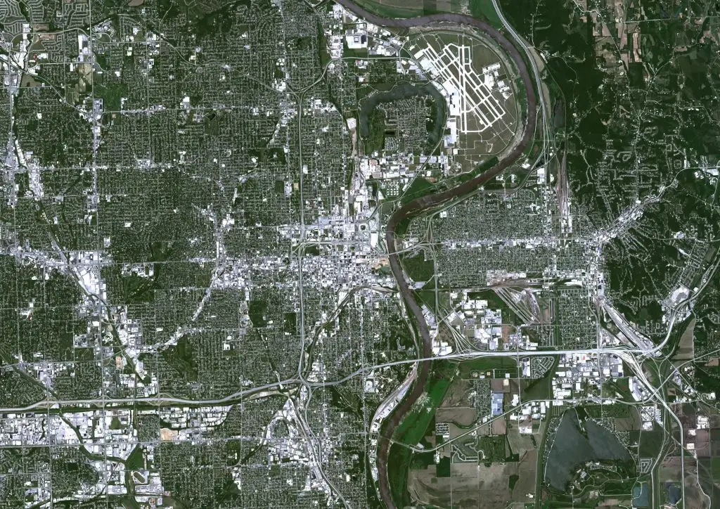

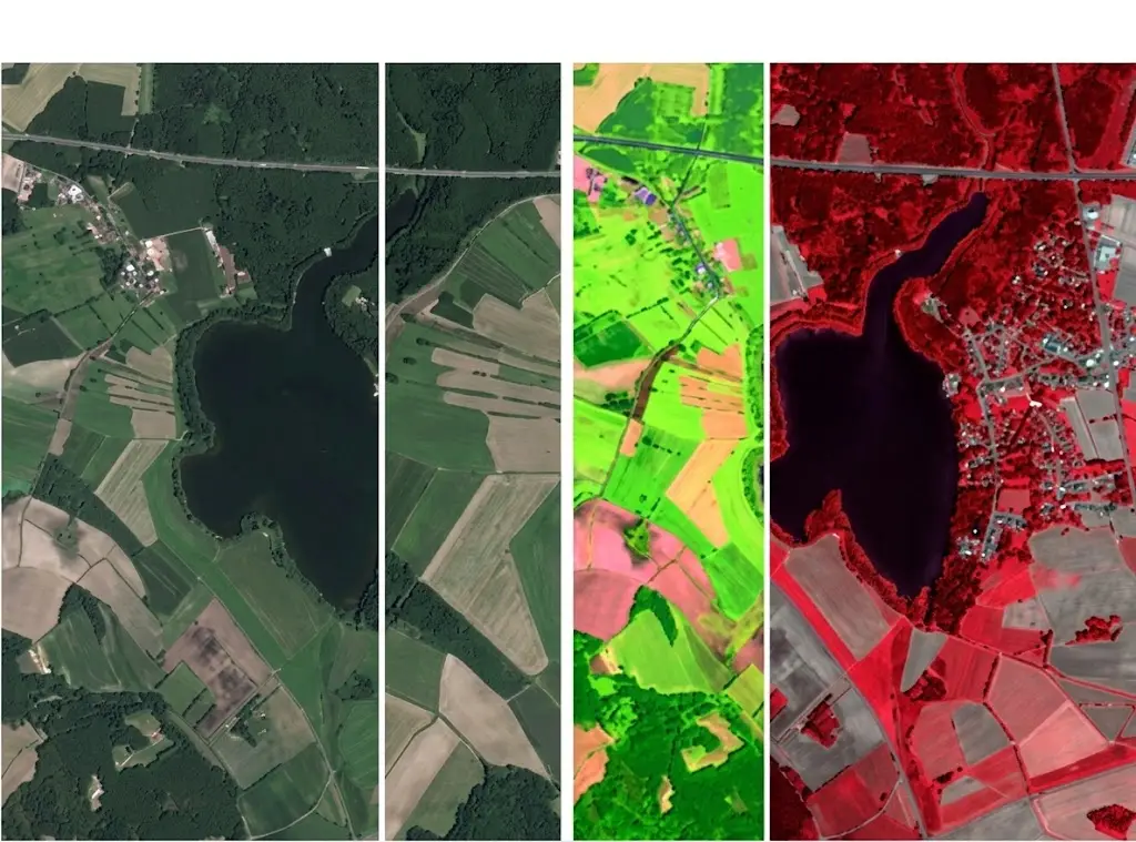
A multispectral sensor records what the eye does not see. The annotator has only their eye, and the whole work consists in making visible information that is not naturally so without distorting it in the process.
This article sets out those methods. It extends the article on agriculture seen from above.
What the bands cover
Six families of spectral band occur in satellite imagery.
The visible, three bands corresponding exactly to human perception.
The near infrared, extremely sensitive to active vegetation.
The mid infrared, sensitive to the moisture held within surfaces.
The thermal infrared, which measures an apparent surface temperature.
The narrow bands that a hyperspectral sensor multiplies.
And the service bands, which are wholly dedicated to atmospheric corrections.
One important practical consequence follows. The second family brings the clearest gain on vegetation, a living plant reflecting very strongly in that particular band, which instantly separates the living from the mineral the visible alone confused.
What the annotator can genuinely see
Four representations make these bands usable in satellite imagery.
A natural colour composite, at once the most legible and the least informative.
A false colour composite, which places the near infrared into the red.
An index image, computed and then displayed in greyscale or in hues.
And the display of one single isolated band shown in greyscale.
One important observation follows for a satellite imagery project. The second representation is the most used on this kind of data, active vegetation appearing there in vivid red, a convention every annotator must learn since it entirely contradicts ordinary visual intuition.
What the choice of composite changes
Four satellite imagery consequences follow from the composite adopted.
It entirely decides what the annotator will notice spontaneously.
It makes certain distinctions obvious and renders others invisible.
It bears directly on consistency between the operators.
And it conditions comparability between two successive batches.
One practical consequence follows. The last consequence justifies fixing the composite at scoping, two batches annotated under different displays producing slightly shifted delimitations without any operator having changed method.
What indices bring
Five computed indices recur constantly in satellite imagery.
A vegetation index, by very far the most used of them all.
A moisture index, sensitive to the water content of surfaces.
A built-up index, which isolates the artificialised spaces.
An open water index, which clearly delimits the water surfaces.
And a bare soil index, particularly useful within an agricultural context.
One observation follows. Those five indices summarise several bands into one value, which makes them immediately legible and makes them lose the information the full combination of bands contained.
What thermal adds
Four uses follow from a thermal band in satellite imagery.
Spotting a heat island within a dense urban environment.
Detecting water stress before it becomes visible at all.
Identifying an industrial installation currently in operation.
And tracking a fire masked by a thick cover of smoke.
One important practical consequence follows for a satellite imagery project. Thermal resolution stays far below that of the visible on most sensors, which limits these uses to extended objects and forbids reasoning at the scale of an isolated building.
What atmospheric correction imposes
Four satellite imagery effects justify this preliminary treatment.
The atmosphere modifies the measured values according to the day’s conditions.
Two uncorrected dates simply do not compare validly.
An index computed on raw values varies with no real cause at all.
And the correction to apply depends on the band considered.
One important observation follows. The second effect touches annotation directly, one same cover showing different hues between two uncorrected acquisitions, which makes the annotator doubt a change that never took place.
What training must cover here
Five points distinguish annotator preparation in multispectral satellite imagery.
The convention of the composite employed along with what each hue signifies.
The appearance of active vegetation, that of bare soil and that of a built surface.
The cases in which false colour misleads rather than actually helps.
The difference between a mere variation in illumination and a real change.
And reading an index image, whose scale is anything but truly intuitive.
One important observation follows for a satellite imagery project. The third point deserves specific time, a metal roof or a shallow water surface producing misleading hues in false colour, which makes certain confusions proper to this representation rather than to the terrain itself.
What the measurement must reflect
Five indicators describe such a satellite imagery system’s performance.
The real contribution of the non-visible bands, measured by direct comparison.
Performance measured by class, some profiting far more than others.
The stability of the results between dates after correction.
The behaviour observed on two different sensors.
And the consistency between operators under a given composite.
One important practical consequence follows. The first indicator deserves establishing before committing the outlay, the contribution of the extra bands varying strongly by class, considerable on vegetation and sometimes nil on manufactured objects.
What the number of bands imposes
Four satellite imagery constraints accompany data with numerous bands.
File weight rises in proportion to the number of bands recorded.
The most common annotation tools handle these formats badly.
Loading time very appreciably slows the work.
And selecting which bands to display becomes a further step.
One important practical consequence follows. The second constraint is better settled at scoping than in production, many tools accepting only three channels, which requires preparing composites upstream rather than letting the annotator explore the bands freely.
What harmonisation between sensors requires
Four gaps separate two multispectral sensors in satellite imagery.
The bands never cover exactly the same wavelengths.
Spatial resolution often differs in notable proportions.
Radiometric values are not expressed on the very same scale.
And revisit frequency varies very strongly between programmes.
One important practical consequence follows for a satellite imagery project. The first gap forbids naively mixing two sources, an index computed on slightly shifted bands giving values that do not compare, which requires a documented harmonisation before any cross annotation.
What these bands permit distinguishing
Five satellite imagery distinctions become possible outside the visible.
Genuinely living vegetation and an artificial green surface.
A moist soil and a dry soil showing the same apparent colour.
An area of open water and a dark cast shadow.
A stressed cover and another cover in good health.
And a built surface and a bare soil showing a neighbouring hue.
One important observation follows for a satellite imagery project. The third distinction resolves a classic confusion of the visible, a shadow and a body of water both appearing dark whereas the near infrared separates them clearly, which appreciably improves land-use corpora.
What this work’s throughput presupposes
Four factors determine the time spent per satellite imagery tile.
The file weight, which slows the loading of each one of the images.
The number of composites to consult before being able to settle.
The operator’s familiarity with the colour convention employed.
And the presence of misleading hues proper to that false colour.
One important practical consequence follows. The third factor improves rapidly then stabilises, an annotator taking a few days to read a false colour with ease, which makes the first week of production markedly less productive than those following on this kind of data.
What the delivery format requires here
Four choices condition the client’s reuse of the satellite imagery result.
The composite employed for annotation, always stated explicitly.
The exact formulas of every one of the indices computed then delivered.
The correction state of the data the work actually bore on.
And identification of the sensor employed, with its bands and their order.
One important observation follows for a satellite imagery project. The second choice avoids costly rework, one same index name covering several formulas depending on the source, which makes a value delivered without its formula impossible to reproduce and therefore hard to contest as much as to defend.
What these data change about quality control
Four difficulties distinguish rereading on this kind of satellite imagery data.
The reviewer sees exactly the same composite as the annotator, so the same traps.
An error due to the representation reproduces identically across all operators.
A control run on the visible bands alone detects none of these errors.
And comparison between operators very poorly reveals a bias they all share.
One important practical consequence follows for a satellite imagery project. The first difficulty justifies a cross-check on a second composite, a reviewer examining the same tiles under a different display spotting errors no ordinary rereading brings out.
What the first batch must establish
Four results justify a satellite imagery trial batch before definitive acquisition.
The performance gap between annotation on visible alone and on full bands.
The composite that annotators judge most legible on this precise terrain.
The list of misleading hues encountered in the composite adopted.
And the time per tile genuinely observed after the learning period.
One important practical consequence follows for a satellite imagery project. The first result settles the chapter’s central question within days, a trial on two hundred tiles sufficing to establish whether the extra bands justify their cost, whereas theoretical discussion of their usefulness can run for weeks without concluding.
What the corpus must cover here
Five axes structure a multispectral dataset built in satellite imagery.
The seasons covered, which strongly modify the response measured in the infrared.
The atmospheric conditions encountered during the various acquisitions.
The sensors employed, whose bands never coincide exactly.
The confusing objects that are proper to the composite finally adopted.
And the classes whose distinction alone motivates using these bands.
One important observation follows. The first axis weighs more here than on visible data, the infrared response of vegetation varying considerably between an active cover and a senescent one, which makes a corpus built within a single season particularly misleading.
What hyperspectral adds and costs
Three contributions separate this satellite imagery sensor from ordinary multispectral.
A very detailed spectral signature rather than a few isolated values.
A distinction rendered possible between materials of neighbouring appearance.
And an identification of chemical composition in some favourable cases.
Three counterparts accompany it in satellite imagery.
Data volume reaches orders of magnitude that are hard to handle.
Availability stays very low and the acquisition remains expensive.
And visual annotation loses its sense, the information no longer being representable in one image.
What this chapter has that is cross-cutting
Three findings from this chapter reach beyond multispectral alone.
Any non-visible data presupposes a representation, and therefore also a choice.
Any summary of rich data loses precisely what its richness contained.
And any extra sensor is justified by a measurement, never on principle.
One important observation follows for a satellite imagery project. Those three findings will apply identically in the chapter on airborne LiDAR, a point cloud being no more annotatable without a chosen representation, which suggests this is a question of method rather than of sensor.
Three errors proper to these data
Three defects appear only on non-visible satellite imagery data.
A misleading hue of the composite, wrongly taken for a field observation.
A gap between two dates attributable to the atmosphere and not to the territory itself.
And an index compared between two sensors with no harmonisation at all.
Those three defects escape any geometric control entirely, they are corrected by method rather than by rereading, and their common point is to come from the processing chain rather than from the annotator themselves.
What the client should ask a provider
Four questions reveal a mastered satellite imagery practice with these data.
Which colour composite they will employ, and for what precise reason.
How they established that these bands served the project’s classes.
Which misleading hues they have already met on comparable terrain.
And how they document index formulas within their deliverables.
One important observation follows for a satellite imagery project. The third question separates them best, a provider able to cite precise confusions having necessarily handled this kind of data, whereas a general answer on the advantages of the near infrared is obtained from any documentation.
What the provider brings here
Four contributions distinguish a multispectral engagement on satellite imagery.
A colour composite carefully chosen then fixed for the whole project.
Annotators trained in all the particular conventions of false colour.
A measurement of the bands’ real contribution before committing any acquisition.
And full documentation of the index formulas employed in the deliverable.
One important practical consequence follows. The third contribution can reduce the client’s invoice, a measurement showing the extra bands bring nothing on their classes saving an expensive acquisition, which builds a confidence selling a larger engagement would not have produced.
Approaching a multispectral project
Five questions scope such a satellite imagery project.
Do the target classes profit from the non-visible bands. Not all do.
Which composite will the annotators see. It decides what they notice.
Are the data corrected for the atmosphere. Otherwise the dates diverge.
Does thermal resolution suffice for the target objects. It is often coarse.
And will the composite stay identical. Otherwise the batches will diverge.
Those five answers determine the arrangement’s real usefulness. Asking them before acquisition avoids paying for extra bands that bring nothing to the case handled.
The question that frames the project
One question determines the arrangement’s usefulness in satellite imagery.
Does what the project seeks to distinguish belong to matter or to form.
A distinction of matter, living or dry vegetation, moist or else dry soil, profits directly from the non-visible bands, which measure a physical property staying inaccessible to the eye.
A distinction of form, one building from another or a road from a mere track, profits in no way from these bands, geometry being observed just as well in the visible.
That question belongs to the nature of the object and not to the sensor, it is asked before acquisition, and it separates a justified investment from an outlay with no return.
Three decisions before producing
Three decisions commit a multispectral project in satellite imagery.
Measuring the real contribution of the non-visible bands on the classes actually targeted.
Fixing the colour composite every annotator on the project will see.
And verifying the data are corrected for the atmosphere before any comparison.
Those three decisions cost one meeting and a simple trial batch, they precede definitive acquisition, and their absence leads to paying for bands that bring nothing to the case handled.
Three checks on a multispectral corpus
Three checks qualify a multispectral dataset in satellite imagery.
The colour composite employed, rigorously identical across all the batches.
The atmospheric correction state of the data actually annotated.
And the measurement of the non-visible bands’ real contribution on the target classes.
Those three checks are each asked in one question, they require no particular competence in remote sensing, and their absence indicates a corpus whose successive batches do not compare with each other.
What this chapter teaches
One cross-cutting observation deserves closing this examination.
Invisible data is annotated only through a chosen representation.
Three findings compose it.
The composite adopted decides what the annotator will notice.
An index summarises several bands and loses what their combination contained.
And the contribution of extra bands varies strongly by target class.
That finding extends the preceding chapter, the agricultural index appearing there as one instance of a more general question.
What this chapter leaves to the next
A network is described neither by a surface nor by a spectral signature.
Three questions stay open in satellite imagery.
How to annotate an object whose length matters far more than its width.
What a continuity interrupted by an obstacle presupposes as a convention.
And how to handle a network passing beneath vegetation or beneath buildings.
Those three questions all belong to infrastructure mapping, which constitutes the subject of the following chapter.
Why measuring the contribution wins the work
One move on this subject is worth more than any capability claim.
Offer to measure whether the extra bands help before anyone buys them.
Three reasons follow in satellite imagery.
Most clients have been sold bands without ever seeing the evidence.
The trial costs a few days and settles a question worth far more.
And the answer is sometimes no, which the client rarely expects to hear.
One important practical consequence follows for a satellite imagery provider. Being willing to reach that answer is itself the argument, since a provider who can say the extra bands are not worth their cost on this particular case has demonstrated something no reference list conveys, and the projects that follow tend to arrive without competition.
Common mistakes
These failures recur often enough that naming them is usually enough to avoid them.
- Acquiring extra bands without measuring their contribution on the target classes.
- Changing colour composite partway through a project.
- Comparing two dates with no atmospheric correction.
- Reasoning on thermal at the scale of an isolated object.
- Confusing an index with the data it summarises.
- Training annotators without explaining the false colour convention.
- Mixing data from different sensors with no harmonisation.
- Neglecting the service bands in the processing chain.
- Applying an index threshold established on another territory.
- Delivering an index without stating its formula or its source.
What to take away
Multispectral shifts the question from observation towards representation.
Three readings emerge. The colour composite adopted decides what the annotator will notice spontaneously, which makes it a methodological parameter to fix at scoping rather than a display setting. An index summarises several bands into one value, a gain in legibility paid for by the loss of the information their combination contained, which forbids confusing it with the data itself. And the contribution of extra bands varies strongly by target class, considerable on vegetation and sometimes nil on manufactured objects, which justifies measuring it before committing the acquisition outlay.
For networks, the article on infrastructure mapping details the approach. For technical preparation, the article on resolution and tiling sets it out.
To explore delivery arrangements, supported formats and applicable control mechanisms, see our dedicated page on annotation for geospatial. And if you are preparing a multispectral project, let us discuss your need.