
Il existe un écart déconcertant entre les performances publiées en détection de défauts et ce que les mêmes méthodes produisent sur une ligne de production. Sur le jeu de données de référence historique du domaine, les approches actuelles atteignent des scores de segmentation situés couramment entre 92 et 97 %, un niveau qui traduit une saturation du jeu de données. Le problème semble donc résolu.
Il ne l’est pas. Sur un jeu de données conçu pour reproduire des conditions plus réalistes, notamment des variations d’éclairage absentes des données d’entraînement, les résultats d’un concours récent tombent à des scores de segmentation compris entre 54 et 63 % selon les jeux de test. Le même type de méthode, la même tâche, et une performance divisée par deux dès que les conditions d’acquisition bougent.
Cet écart est le sujet central de la détection de défauts industrielle, et il se joue en grande partie avant l’algorithme : dans la définition de ce qu’est un défaut, dans la constitution du jeu de données et dans la façon dont il est annoté. Ce guide couvre l’ensemble du domaine, des approches disponibles aux tâches d’annotation, en passant par les capteurs, l’ontologie et le contrôle qualité.
Ce que recouvre la détection de défauts par vision
Le terme de détection de défauts désigne l’usage de la vision par ordinateur pour identifier, localiser ou qualifier une anomalie sur un produit, un composant ou une surface, en vue d’une décision de conformité. Cette définition large recouvre des situations assez différentes.
Défaut, anomalie, non-conformité
Le vocabulaire courant mélange trois notions qui n’ont pas les mêmes conséquences pratiques, et il vaut la peine de les séparer avant tout le reste. Trois notions se confondent souvent et gagnent à être distinguées. Une anomalie est un écart par rapport à l’apparence attendue, indépendamment de sa gravité. Un défaut est une anomalie identifiée comme telle par un référentiel qualité. Une non-conformité est un défaut qui dépasse un seuil de tolérance et déclenche une décision : rebut, retouche, déclassement.
Cette distinction n’est pas académique. Elle détermine ce que le modèle doit produire. Un système d’anomalie signale ce qui sort de l’ordinaire sans le nommer. Un système de détection de défauts nomme et localise. Un système de contrôle décide. Les trois exigent des annotations différentes, et confondre les niveaux au moment du cadrage est l’erreur la plus fréquente du domaine.
Défauts structurels et défauts logiques
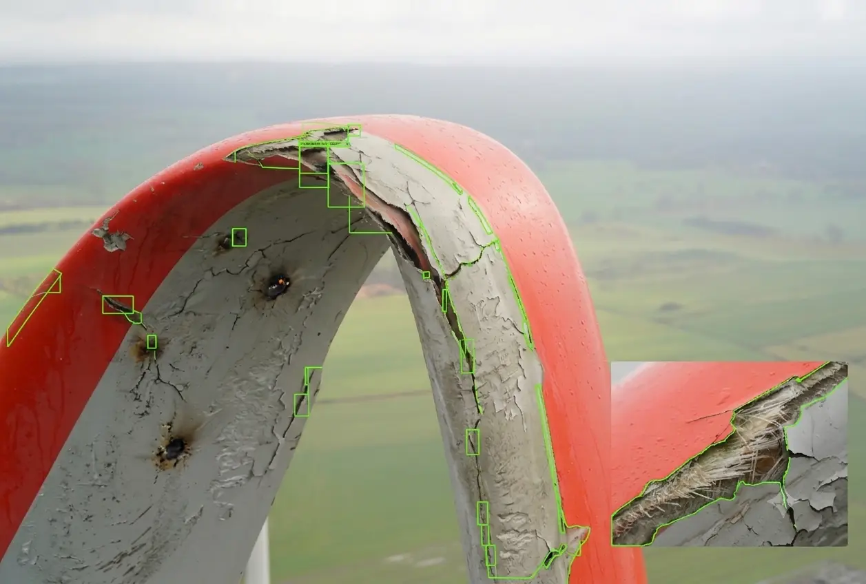
Une seconde distinction, plus récente, sépare les défauts structurels des défauts logiques. Un défaut structurel est une altération locale de la matière : rayure, fissure, tache, manque, inclusion. Un défaut logique concerne l’agencement : une pièce absente, un composant en trop, un ordre incorrect, une couleur inattendue dans un assemblage par ailleurs correct. Les méthodes efficaces sur les premiers échouent souvent sur les seconds, parce qu’un défaut logique n’a pas de signature locale et ne se voit qu’à l’échelle de l’objet entier.
Pourquoi c’est un problème différent de la vision généraliste
Trois caractéristiques distinguent la détection de défauts de la reconnaissance d’objets classique, et chacune a des conséquences directes sur la constitution du jeu de données.
Le déséquilibre extrême
Sur une ligne maîtrisée, le taux de défaut se compte en fractions de pour cent. Constituer un jeu d’entraînement équilibré supposerait de parcourir des volumes considérables de pièces conformes pour rassembler quelques centaines d’exemples défectueux, et certaines catégories de défauts n’apparaîtront que quelques fois par an. C’est le problème central du domaine, et il conditionne le choix des approches autant que la stratégie d’annotation.
Le défaut inconnu
Un système de reconnaissance d’objets connaît la liste de ce qu’il doit trouver. Un système de détection de défauts, non : un nouveau mode de défaillance peut apparaître à tout moment, lié à un changement de matière première, d’outillage ou de réglage. Un modèle entraîné à reconnaître les défauts connus ne signalera pas un défaut d’un type nouveau, et ce silence est plus dangereux qu’une fausse alerte.
La tolérance plutôt que la classe
En vision généraliste, un objet appartient ou non à une classe. En contrôle industriel, un même type de défaut est acceptable en dessous d’une certaine taille et rédhibitoire au-dessus, et le seuil dépend de la zone de la pièce, de sa destination et parfois du client final. L’annotation doit donc porter non seulement sur la nature du défaut mais sur les attributs qui permettent d’appliquer la règle de tolérance.
Les grandes familles d’approche
Quatre familles d’approche coexistent en détection de défauts, et le choix dépend directement de la disponibilité d’exemples défectueux.
Les méthodes classiques
Seuillage, morphologie, corrélation avec un gabarit, mesure dimensionnelle : ces approches restent pertinentes lorsque le défaut est géométriquement défini et l’environnement parfaitement maîtrisé. Elles sont rapides, explicables et ne demandent pas de jeu de données. Elles deviennent inopérantes dès que l’apparence normale varie, ce qui est le cas de la plupart des surfaces réelles.
L’apprentissage supervisé
Classification, détection ou segmentation entraînées sur des exemples annotés de chaque type de défaut. C’est l’approche la plus performante lorsque les exemples existent en nombre suffisant, et la plus exigeante en annotation. Elle suppose de connaître à l’avance la liste des défauts, ce qui la rend vulnérable aux modes de défaillance nouveaux.
La détection d’anomalie non supervisée
C’est l’approche qui a le plus progressé récemment, et elle répond directement au problème du déséquilibre. Le modèle apprend uniquement sur des exemples conformes et signale tout écart. Les jeux de données de référence du domaine sont conçus sur ce principe : le jeu de référence historique comprend 5 354 images haute résolution réparties en 15 catégories, dont 10 classes d’objets et 5 classes de textures, avec des anomalies couvrant plus de 70 types de défauts tels que rayures, bosses et contaminations, chaque catégorie fournissant un ensemble d’entraînement composé d’images sans défaut.
L’avantage est décisif : constituer un jeu de pièces conformes est trivial sur une ligne en fonctionnement. La contrepartie est que le système signale sans nommer, et qu’il déclenche des alertes sur des variations normales mais inhabituelles, ce qui pose un problème d’acceptation en production.
Les approches hybrides
En pratique, les déploiements matures combinent les deux logiques : une détection d’anomalie pour la couverture large, y compris des défauts inconnus, et un modèle supervisé pour classer et qualifier les défauts fréquents dont on dispose d’exemples. Cette architecture demande une stratégie d’annotation à deux niveaux, et elle est nettement plus robuste qu’une approche unique.
Capteurs et conditions d’acquisition
En détection de défauts, la qualité de l’acquisition pèse davantage sur le résultat final que le choix de l’architecture, et c’est le poste où un projet se gagne ou se perd.
L’éclairage
C’est le paramètre dominant. Un éclairage rasant révèle les défauts de relief, un éclairage diffus révèle les défauts de couleur, un éclairage en champ sombre révèle les rayures fines. Un même défaut peut être parfaitement visible sous un montage et invisible sous un autre. Concevoir l’éclairage en fonction des défauts recherchés, plutôt que d’espérer qu’un algorithme compense, est la décision la plus rentable d’un projet de détection de défauts.
La stabilité de cet éclairage compte autant que sa conception. Les résultats évoqués en introduction le montrent : c’est précisément l’introduction de variations d’éclairage entre entraînement et test qui fait chuter les performances de moitié. En production, la lumière ambiante, l’empoussièrement des optiques et le vieillissement des sources produisent exactement ce type de dérive.
Les modalités
Le choix de la modalité découle de la nature physique du défaut recherché. L’imagerie couleur ou monochrome couvre la majorité des cas. L’imagerie tridimensionnelle, par profilométrie ou stéréovision, s’impose lorsque le défaut est un écart de forme plutôt que d’apparence. La thermographie révèle des défauts internes ou des anomalies de process. La radiographie détecte les inclusions et les porosités invisibles en surface. Chaque modalité appelle des conventions d’annotation propres, et un projet multimodal doit maintenir des ontologies articulées mais distinctes.
La cadence
La vitesse de défilement contraint le temps d’exposition, donc l’éclairage, et impose une limite au temps d’inférence disponible par pièce. Ces contraintes se fixent en amont et déterminent des choix techniques irréversibles, ce qui justifie de les documenter dès le cadrage plutôt que de les découvrir à l’intégration.
Les tâches d’annotation en détection de défauts
Cinq formats de sortie structurent les projets de détection de défauts, avec des coûts et des usages très différents.
La classification au niveau de l’image indique la présence ou l’absence d’un défaut, éventuellement son type. C’est la plus rapide à produire et la moins informative, puisqu’elle ne dit pas où regarder. La boîte englobante localise grossièrement, ce qui suffit au tri et à l’alerte. Le polygone ou le masque pixel délimite le défaut précisément, seule solution lorsque la surface ou la longueur du défaut entre dans la règle de tolérance. Le comptage s’applique aux défauts multiples, porosités ou inclusions, avec les exigences propres aux tâches de dénombrement. Enfin, l’annotation d’attributs qualifie chaque défaut au-delà de son type : gravité, profondeur estimée, zone de la pièce concernée.
Le choix ne relève pas de la préférence technique : il se déduit de la règle de décision qualité. Si la règle stipule qu’un défaut de plus de deux millimètres dans une zone critique est rédhibitoire, l’annotation doit permettre de mesurer la taille et d’identifier la zone, ce qui exclut la simple classification. Partir de la règle qualité pour définir la primitive, plutôt que l’inverse, évite de produire un corpus qui ne permet pas de trancher.
Construire l’ontologie des défauts
C’est le travail le plus déterminant d’un projet de détection de défauts, et le plus souvent expédié.
Nommer par apparence ou par cause
Les équipes qualité nomment les défauts par leur cause : défaut de soudure, problème de refroidissement, dérive d’outil. Un modèle de vision ne voit que l’apparence, et deux causes différentes peuvent produire des images indiscernables. Une ontologie construite sur les causes produit donc des classes que le modèle ne peut pas séparer, et un accord entre annotateurs médiocre.
La solution consiste à construire une ontologie à deux niveaux : un niveau d’apparence, annotable de façon fiable à partir de l’image seule, et un niveau de cause, renseigné lorsque l’information est disponible par ailleurs. Les deux se relient, et le corpus reste exploitable pour la maintenance comme pour le contrôle.
La gravité
La gravité est ce qui relie l’observation à la décision, et sa définition mérite autant de soin que la liste des classes. Une échelle de gravité doit être définie avec des critères objectifs, taille, position, contraste, plutôt qu’avec des qualificatifs comme léger, moyen ou important. Une échelle subjective produit une variabilité considérable entre annotateurs, et cette variabilité se retrouve directement dans le comportement du modèle aux abords du seuil de décision, c’est-à-dire exactement là où il compte.
Les classes de service
Trois classes techniques sont indispensables. Une classe pour les images de qualité insuffisante, avec des critères explicites. Une classe pour l’incertitude assumée, qui vaut mieux qu’une décision forcée. Et une classe pour les anomalies visibles mais non répertoriées, qui est le canal par lequel les modes de défaillance nouveaux remontent à l’équipe qualité.
Le piège des jeux de données publics
Les jeux de référence en détection de défauts sont précieux pour comparer des méthodes, et trompeurs si l’on en déduit une performance attendue en production.
Les conditions y sont contrôlées, les catégories peu nombreuses et l’apparence normale peu variable. Les jeux plus récents corrigent partiellement ce biais : l’un d’eux ajoute huit scénarios comportant plus de 8 000 images haute résolution, avec des données de test capturées sous des conditions d’éclairage variées qui ne figurent pas nécessairement dans les données d’entraînement, et une vérité terrain non publique pour une partie du test évaluée uniquement via un serveur.
La conclusion pratique est qu’un chiffre de performance publié n’a de valeur que rapporté à ses conditions. Avant de s’engager sur un objectif, il faut mesurer sur ses propres données, dans ses propres conditions d’éclairage, avec sa propre variabilité de production.
Le contrôle qualité d’une annotation de détection de défauts
Un corpus de détection de défauts présente une difficulté de contrôle spécifique : la vérité est parfois indécidable à partir de l’image seule.
Un opérateur expérimenté hésite parfois, et cette hésitation est une information à conserver plutôt qu’un problème à supprimer. Trois mécanismes se combinent. La double lecture indépendante sur les classes à faible accord, généralement les défauts fins et les cas proches du seuil de gravité. L’arbitrage par un expert qualité, dont les décisions doivent être documentées et rediffusées, chaque arbitrage créant une jurisprudence applicable à des centaines de cas. Et l’insertion de cas de référence dans le flux de production, qui mesure la dérive individuelle sur une tâche répétitive et fatigante.
Les métriques doivent être rapportées par classe et non en agrégat. Sur un corpus déséquilibré, un indicateur global est dominé par les images conformes et reste excellent alors que la détection des défauts rares s’effondre. Il faut également distinguer explicitement les omissions des fausses détections, qui n’ont ni les mêmes causes ni les mêmes conséquences industrielles : une omission laisse partir une pièce non conforme, une fausse détection dégrade le rendement.
Le coût et les profils d’annotation
Un projet de détection de défauts présente un profil de coût inhabituel, dominé non par le volume mais par la rareté.
Le temps passé à parcourir des images conformes pour atteindre les exemples défectueux constitue souvent le poste principal, ce qui rend le prétri par un modèle ou par une règle simple particulièrement rentable. Le contrôle qualité pèse également lourd, parce que les cas litigieux sont fréquents et que leur arbitrage mobilise un expert qualité dont le temps est rare.
La répartition des rôles est en revanche favorable. Le repérage et la délimitation d’un défaut visible relèvent d’une décision perceptive et se délèguent bien à des annotateurs formés, à condition que le protocole soit précis et illustré. La qualification de la gravité, la décision de conformité et l’arbitrage relèvent de l’expert qualité. Une chaîne bien organisée réserve son temps à ces trois usages et lui évite le parcours des images conformes.
Du prototype à la ligne
Un projet échoue rarement au stade de la faisabilité et souvent au stade de l’industrialisation. Quatre écarts expliquent la plupart de ces échecs.
La dérive des conditions d’acquisition, déjà évoquée, est la première. La dérive du produit vient ensuite : un changement de fournisseur de matière, de teinte ou de process modifie l’apparence normale et déclenche des alertes injustifiées. Le troisième écart tient à l’acceptation par les opérateurs, qui cessent de tenir compte d’un système générant trop de fausses alertes. Le quatrième tient à l’absence de boucle de retour : sans mécanisme permettant à l’opérateur de signaler une erreur du système et de la faire remonter dans un corpus de correction, le modèle se dégrade sans que personne ne le mesure.
Ces quatre écarts ont en commun de ne pas être des problèmes d’algorithme, ce qui explique qu’ils échappent aux phases de validation technique. La parade est une conception qui prévoit dès le départ la collecte continue, l’annotation périodique des cas litigieux et le réentraînement. Un système de vision industrielle n’est pas un produit livré une fois, c’est une capacité entretenue.
Les secteurs et leurs spécificités
Les principes de détection de défauts exposés ici valent partout, mais chaque secteur infléchit la difficulté sur un point précis.
Dans la métallurgie et la transformation de surface, le défi tient à la variabilité de l’aspect normal : brillance, texture, traces d’usinage produisent un fond très bruité sur lequel les défauts fins sont difficiles à isoler. Dans l’électronique et l’assemblage, la difficulté se déplace vers les défauts logiques, absence, inversion ou substitution de composant, qui demandent une compréhension de l’agencement plutôt qu’une analyse locale. Dans le textile et les matériaux souples, la déformation de la pièce entre deux acquisitions interdit toute comparaison à un gabarit et impose des méthodes tolérantes à la géométrie. Dans l’agroalimentaire, la variabilité naturelle du produit est telle que la frontière entre variation acceptable et défaut devient une décision commerciale autant que technique.
Cette diversité explique qu’aucune solution générique ne s’installe sans travail de cadrage. La partie transférable d’un projet à l’autre est la méthode, pas le modèle.
Les erreurs les plus fréquentes
- Construire l’ontologie sur les causes plutôt que sur l’apparence visible.
- Définir la gravité par des qualificatifs subjectifs sans critères mesurables.
- Choisir la primitive d’annotation sans partir de la règle de décision qualité.
- Extrapoler une performance publiée sur un jeu de référence à ses propres conditions.
- Négliger la conception de l’éclairage en comptant sur l’algorithme pour compenser.
- Rapporter une exactitude globale sur un corpus fortement déséquilibré.
- Confondre omissions et fausses détections dans un indicateur unique.
- Ne prévoir aucune classe pour les anomalies visibles mais non répertoriées.
- Livrer un système sans boucle de retour ni plan de réentraînement.
Ce qu’il faut retenir
La détection de défauts est un domaine où la performance publiée et la performance obtenue divergent fortement, et où l’écart s’explique presque entièrement par des facteurs que l’algorithme ne contrôle pas : la stabilité de l’acquisition, la définition des classes, la représentativité du corpus et la clarté de la règle de décision.
Trois décisions font l’essentiel. Concevoir l’éclairage et l’acquisition en fonction des défauts recherchés, avant de choisir une méthode. Construire une ontologie fondée sur l’apparence, avec une échelle de gravité à critères mesurables. Et prévoir dès la conception la boucle de collecte, d’annotation et de réentraînement qui permettra au système de suivre les évolutions du produit et de la ligne.
Pour l’intégration concrète en environnement de production, l’article consacré au contrôle qualité automatisé sur ligne de production détaille les questions de cadence, d’éclairage et de tolérances. Pour le problème central du déséquilibre de classes, l’article sur l’annotation des défauts rares couvre les stratégies de rééchantillonnage et de données synthétiques.
Pour approfondir les modalités d’exécution, les formats pris en charge et les dispositifs de contrôle applicables, vous pouvez consulter notre page dédiée à l’annotation pour l’industrie. Et si vous préparez un corpus d’inspection et souhaitez cadrer l’ontologie et la stratégie d’annotation avant de lancer la production, échangeons sur votre projet.