

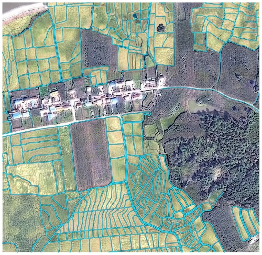
The opening article of this series on satellite image segmentation announced that most annotator disagreement and most model error concentrates on boundary pixels. The articles devoted to the individual classes confirmed it in varied forms.
This one addresses the question directly: why boundaries concentrate the difficulty, why the usual metrics mask it, and how a project can handle it. It extends the article on hyperspectral segmentation.
Why the boundary concentrates the difficulty
Four mechanisms combine at the limits of an object. They explain the entirety of the phenomenon. The mixed pixel comes first among those mechanisms. A pixel straddling two classes records a mixture of their signatures, which makes assigning it to either one arbitrary by nature. The physical transition comes next. Many real limits are not sharp, a forest edge or a shoreline presenting a zone of gradation where no position imposes itself. Convention intervenes third. Even on a sharp limit, whether the line runs at the edge, through the middle or beyond an element is a decision observation does not settle. And georeferencing imprecision intervenes fourth. An offset of a fraction of a pixel between imagery and reference produces systematic disagreement on every boundary without any interpretive error having been made. Those four mechanisms share a decisive common property. None is corrected by a better model, the first three belonging to the data and the convention, the fourth to a geometric problem upstream.Why the usual metrics mask it
An arithmetic property makes it invisible in an ordinary evaluation. A compact region contains far more interior pixels than boundary pixels, and that ratio grows with the size of the object. A parcel one hundred metres across at ten metre resolution contains one hundred pixels of which thirty-six lie on the perimeter; the same parcel at one metre resolution contains ten thousand of which three hundred and ninety-six. One direct consequence follows. The finer the resolution, the smaller the proportion of boundary pixels, and the less sensitive a global metric becomes to the quality of the limits. Three effects follow directly for a satellite image segmentation project. High global performance is compatible with mediocre contours. An improvement in boundary quality registers as a marginal gain on the metric, which discourages the effort. And two models with identical scores can produce contours of very different quality. That third effect is the most problematic commercially. A client comparing two offerings on a single score does not see the difference that will determine their use.Boundary-sensitive metrics
Four measures evaluate what global metrics ignore. It is worth distinguishing them. The boundary score restricts the computation to a narrow band either side of the reference contour, which excludes interior pixels and makes the measure directly sensitive to what matters. Contour distance measures the mean geometric discrepancy between predicted and reference contours, expressed in ground units rather than as a proportion of pixels, which makes it interpretable by a client. Maximum distance, or a truncated version discarding extreme values, measures the worst discrepancy rather than the average, useful information where a single error matters. And parameterised tolerance evaluates the proportion of predicted contour lying within a given distance of the reference, which permits expressing a requirement in operational terms. One recommendation follows. Reporting a global metric alongside a boundary metric gives a picture neither supplies alone, and that double measurement costs one additional computation.The bound imposed by the reference
This theoretical limit bounds everything above. Two competent annotators do not trace exactly the same limit. Their disagreement is a measure of the reference’s noise, and no model can do better than that noise. Three consequences follow for an annotated project. A precision requirement below the inter-annotator disagreement is unachievable, whatever the method. A model reaching that level cannot be improved further without first improving the reference. And a measured discrepancy between prediction and reference below that noise has no meaning. One important methodological consequence follows. Measuring inter-annotator disagreement on boundaries, separately from global disagreement, supplies the relevant bound and that measurement is rarely made. That measurement has direct commercial value. It permits answering an unrealistic precision requirement with a fact rather than a negotiation, which moves the conversation onto verifiable ground.The role of georeferencing
This source of error is frequently confused with a satellite image segmentation error. An offset between the annotated imagery and the production imagery produces a systematic contour discrepancy, identical on every object and in the same direction. Three signs clearly distinguish it from a model error. The discrepancy is constant in direction and amplitude across a whole area. It is uncorrelated with object type or case difficulty. And it disappears if the two sources are registered before comparison. One practical consequence follows. Verifying alignment before any quality diagnosis avoids attributing to a model an error belonging to a geometric problem, a situation the buildings article flagged as dominant in change detection. That verification takes minutes and it is regularly omitted, which leads teams to attempt improving a model that works correctly.The conventions that determine quality
A substantial part of boundary variability belongs to decisions not taken rather than to errors committed. Five questions must be settled explicitly and documented with illustrations. The position of the limit on a gradual transition, which calls for a quantified criterion rather than a judgement. The treatment of the mixed pixel, assigned to the dominant class, to a transition class or under a proportion threshold. The treatment of boundary elements, hedgerow, bank, verge or roof overhang, whose inclusion is a matter of convention. The degree of smoothing expected, a contour following every irregularity and a regularised contour not expressing the same thing. And the treatment of adjacent shadowed areas, where the real limit is invisible and must be interpolated or flagged. One observation runs across those five questions. Each is settled in minutes with an expert and produces, if omitted, a variability nothing can subsequently distinguish from real error.The effect of resolution on achievable precision
This relationship is often misunderstood. It determines what a satellite image segmentation project can promise. Contour precision cannot fall below the pixel size, and in practice it approaches it only with difficulty. Three factors explain that. The pixel is the indivisible unit of measurement, which mechanically bounds precision. The mixed pixel spreads the transition over at least one pixel either side. And any resampling, during a geometric correction, introduces additional blur. One practical rule follows. A contour precision on the order of one to two pixels is a correct result, and a lower requirement presupposes either finer resolution or a complementary source. That rule has a direct commercial consequence. It permits translating a ground requirement into a resolution requirement, and therefore into an acquisition budget, which moves a quality discussion towards a discussion of means.What the model can contribute
Several techniques genuinely improve contour quality and it is worth situating them. Weighted loss functions give greater weight to boundary pixels, which offsets their low proportion and directs learning towards them. Contour terms add a geometric discrepancy measure to the learning, which explicitly penalises a misplaced contour independently of its pixel cost. Resolution-preserving architectures avoid the loss of fine information that compression causes, a difficulty the models article details. And two-stage refinement produces a coarse segmentation first then refines the contours, which concentrates computation where it is useful. One important caveat accompanies those four techniques. All presuppose a reference whose contours are reliable, failing which they learn to reproduce the annotation’s noise faithfully, which worsens the situation rather than improving it.What post-processing can contribute
Three operations improve a contour after prediction and their effects differ. Smoothing removes pixel-level irregularities, which improves appearance and can degrade precision if the real contour is genuinely irregular. Geometric regularisation imposes an expected shape, right angles for buildings notably, which the corresponding article detailed with its caveats. And alignment onto an existing reference constrains the predicted contour to coincide with a known limit, parcel layer or network, where such a reference exists. One consequence for evaluation deserves stating. Those three operations modify the metrics, sometimes downwards while the product is better for the use, which requires measuring before and after and documenting the parameters.Annotating boundaries in practice
Four practices improve contour quality in satellite image segmentation. They cost little and are put in place immediately. Systematic zooming at limits, an annotator working at overview scale producing markedly less precise contours than the same annotator working at maximum zoom on the boundaries. Displaying several colour compositions, a limit invisible in one band combination sometimes appearing clearly in another. Edge-assisted tracing, which proposes a line following the image gradients for the annotator to correct, improving both speed and regularity. And double reading of difficult cases, two annotators independently handling the configurations identified as ambiguous with a third arbitrating the discrepancies. That fourth practice deserves targeting rather than generalising. Applied across a whole corpus it doubles the cost, applied only to difficult configurations it raises it marginally and it addresses precisely where variability concentrates. One observation completes those four practices. None compensates for the absence of a documented convention, a precise annotator applying a rule they invented producing a contour consistent with themselves and inconsistent with their colleagues.How to express a precision requirement
An operational formulation is better than a score requirement and it is built in three steps. Establish first what the imprecision costs the client. A one-metre discrepancy on a parcel limit may represent a chargeable area; the same discrepancy on a forest edge may have no consequence at all. Translate that cost next into a tolerance expressed in ground units, a formulation a client understands and a supplier can verify. And verify finally that the tolerance exceeds the measured inter-annotator disagreement, failing which the requirement is unachievable and should be renegotiated before rather than after. That approach usefully replaces a score requirement whose concrete implications nobody knows. It produces a verifiable criterion and it protects both parties.Boundary-targeted quality control
This method differs from an ordinary sampling. A check by random area sampling is dominated by easy cases, the interior of objects constituting most of the surface. A targeted check preferentially examines boundary zones and, among them, the configurations identified as difficult: gradual transitions, adjacency between neighbouring classes, shadowed areas and small objects. Three measurable benefits follow. The error detection rate is markedly higher at constant effort. The errors found are those affecting the use. And the disagreements reveal convention gaps rather than individual failings. One caveat accompanies that method. An exclusively targeted check says nothing about overall quality, which argues for a combination, a light random sample and a denser targeted one.What boundaries cost in satellite image segmentation
The precision requirement is a project’s principal cost lever. Three lines grow with the precision demanded. Annotation time, a contour traced at maximum zoom taking several times that of an approximate one, the gap being sharper than on any other requirement. Checking, high precision presupposing the targeted double reading described above. And acquisition, a requirement exceeding what the resolution permits imposing a finer source, which is the heaviest line. One practical consequence follows. Halving a precision requirement does not halve the cost but divides it further, the relationship not being linear, which makes that negotiation particularly fruitful at scoping. One observation completes that. A client frequently asks for precision above their real need, out of caution, and the exercise of translating the requirement into operational cost generally leads to a voluntary revision, which improves the value to cost ratio without degrading the use.Demonstrating contour quality
One commercial difficulty deserves addressing, a provider producing good contours being unable to show it by the usual means. Four demonstrations respond to that and they are prepared in advance. Visual comparison at high zoom on difficult cases, which makes immediately perceptible a difference the figures do not show. The boundary measure reported alongside the global metric, with an explanation of what it means, which installs the subject in the discussion. Contour distance expressed in metres, which speaks to a client used to reasoning in ground precision rather than in pixel proportions. And the inter-annotator disagreement measure, which situates the performance obtained relative to what is achievable rather than to a theoretical ideal. That fourth demonstration is the most convincing and the least practised. It shows that a result close to the human bound cannot be significantly improved, which answers in advance the question of whether a competitor would do better.What this means commercially
Three commercial consequences emerge for a satellite image segmentation provider. The first is that contour quality is a differentiator invisible in a global score. A provider producing markedly better contours than a competitor cannot demonstrate it through the usual metric, which argues for proposing a boundary measure in any comparison. The second is that measuring inter-annotator disagreement on boundaries is a deliverable in itself. It establishes what is achievable, it protects against an unrealistic requirement and it demonstrates a methodological command few suppliers display. And the third is that documented conventions are worth more than announced performance. A corpus whose boundary rules are written and illustrated can be reused, extended and defended, where a corpus produced without them permits none of those three.Why this question runs through the whole series
This observation connects the eight preceding articles. It closes the examination of the classes and modalities of satellite image segmentation. Each class examined met this difficulty in its own form. Water meets it on gentle banks, where the transition is gradual. Buildings meet it on roof overhangs and party walls. Vegetation meets it on forest edges. Linear objects meet it everywhere, their boundary to interior ratio being extreme. Radar aggravates it through speckle, which blurs limits. And hyperspectral displaces it towards the mixed pixel, which is a boundary seen from composition. That recurrence is not a coincidence. It reflects a property of the operation itself: segmentation imposes discrete limits on a continuous reality, and the price of that imposition is paid exactly where the continuity was real. One general consequence follows for a project. The most profitable methodological effort concerns neither the model nor the volume, but the boundary conventions, which cost days and determine the ceiling of everything after.When boundary precision does not matter
One satellite image segmentation qualification deserves making, since an article devoted to precision risks suggesting that more is always better. Several uses tolerate imprecise contours entirely, and pursuing precision there wastes budget without improving anything. Area statistics over a wide territory tolerate boundary error well, since discrepancies in both directions partly cancel across many objects, an effect the validation article in the previous series covered from the estimation angle. Presence detection tolerates it completely, since the question is whether an object exists rather than exactly where it ends. Trend monitoring tolerates a systematic bias, since a consistent error affects both dates equally and cancels in the comparison, provided the bias really is consistent. And coarse zoning tolerates it by construction, the delivered product being aggregated well above the pixel scale. One practical consequence follows. Establishing early whether the use falls into one of those four categories can remove the most expensive requirement of a project at no cost to the client, which is a rarer conversation than the reverse and a more welcome one.Common mistakes
These failures recur often enough that naming them is usually enough to avoid them.- Relying on a global metric to judge contour quality.
- Comparing two models on a single score with no boundary measure.
- Attributing to a model an offset belonging to georeferencing.
- Setting a precision requirement below the inter-annotator disagreement.
- Not measuring that disagreement separately on boundaries.
- Using weighted loss functions on a noisy reference.
- Smoothing a contour without checking the effect on precision.
- Omitting to document boundary conventions.
- Checking quality by random area sampling.
- Expressing a requirement as a score rather than as a ground tolerance.
- Annotating boundaries at overview scale rather than at zoom.
- Requiring a precision below the pixel size.