
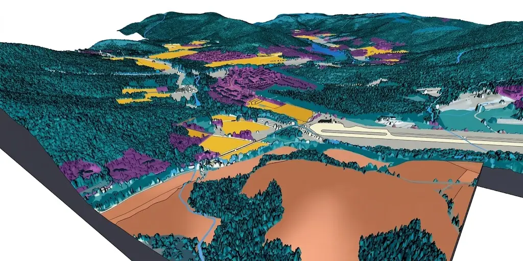
A point cloud is not an image. Nothing in it can be looked at without first choosing a viewpoint, a colouring and a display mode, and that absence of any natural representation changes the whole annotation work.
This article sets out those methods. It extends the article on natural disasters.
What this sensor produces
Five characteristics separate this data from an ordinary satellite image.
Every point carries three directly measured coordinates.
Point density varies strongly with the surface encountered.
Several returns sometimes come from one same pulse.
Signal intensity also reports on the nature of the material.
And no natural order truly organises the set of points.
One important practical consequence follows. The third characteristic explains this sensor’s major interest, a first return coming from the foliage and a last one from the ground, which permits seeing beneath vegetation where optical imagery shows only the canopy.
The uses that structure the field
Six LiDAR applications occur in satellite imagery.
Producing a terrain model established beneath the vegetation.
Measuring the height of buildings as well as of structures.
Forest inventory as well as biomass estimation.
The precise modelling of flood-prone areas.
Spotting archaeological remains concealed beneath canopy.
And detecting ground movement occurring between two campaigns.
One important observation follows. The fifth use is specific to this sensor, a low mound invisible beneath the trees appearing clearly once the vegetation is removed from the cloud.
What classifying the points requires
Six classes compose a nomenclature common to satellite imagery and airborne work.
The ground, which serves as the base of any terrain model.
The vegetation, most often split into height strata.
Built form, distinguished from the ground by its elevation alone.
The water, whose laser return remains very particular.
The linear structures, such as bridges and power lines.
And the outlier points, which must be discarded from processing.
One practical consequence follows. The first class conditions all the others, a ground classification error propagating into every height computed by difference, which makes it the object of the most attentive control.
What the annotator must see
Five representations make a satellite imagery point cloud usable.
A perspective view, which one is free to orient at will.
A top-down view, coloured according to the elevation.
A vertical cross-section, which at once reveals the structure.
A colouring established by the return intensity.
And a colouring by class having already been assigned.
One important observation follows for a satellite imagery project. The third representation is the most discriminating and the least employed, a cross-section showing immediately the stratification neither the top-down view nor the perspective renders legible.
What this work’s throughput presupposes
Five factors separate this work from classic satellite imagery annotation.
Navigating in space consumes a time all of its own.
The data volume appreciably slows every manipulation.
Selecting a set of points demands a great deal of precision.
Changing viewpoint comes to interrupt the gesture.
And learning the tool extends across several weeks.
One important practical consequence follows. The last factor weighs heavily on a first project, a team competent in image annotation nonetheless staying a novice before a point cloud, which makes the ramp-up far slower than anticipated.
What the reference requires here
Four sources establish an elevation ground truth in satellite imagery.
The topographic surveys carried out directly on the ground.
Direct measurements conducted on a sample of objects.
Terrain models already existing over the area.
And expertise conducted by a surveyor or by a forester.
One observation follows. The first source reaches an accuracy far above that of the cloud, which makes it a solid reference on a restricted sample and a means of measuring the error rather than of correcting it.
What fusion with the image brings
Five benefits follow from a cloud coloured by a satellite imagery image.
Classification becomes markedly safer on the ambiguous surfaces.
The annotator finally recovers familiar visual landmarks.
The distinction between built form and tall vegetation is confirmed.
Checking the result becomes accessible to a non-specialist.
And the deliverable then serves both measurement and interpretation.
One important practical consequence follows. The second benefit appreciably reduces the learning period, a coloured cloud reading far faster than one in elevation shades, which softens the entry barrier this sensor sets against teams coming from image annotation.
What the measurement must reflect
Five indicators describe the quality of a classified point cloud.
The accuracy of the ground classification itself.
The elevation gap observed against measured reference points.
The consistency obtained between adjacent flight lines.
The performance obtained over areas of particularly dense canopy.
And the proportion of points finally left unclassified.
One important practical consequence follows. The fourth indicator deserves isolating, ground point density falling sharply beneath a closed canopy, which makes the terrain model less reliable the denser the forest, precisely where it was most expected.
What comparison between campaigns requires
Four conditions make two satellite imagery acquisitions comparable.
A precise registration of the two clouds carried out on fixed points.
A comparable point density between each of the two dates.
A ground classification conducted by the same method.
And an equivalent season for all the vegetated areas.
One important observation follows for a satellite imagery project. The first condition determines all the rest, a registration gap of a few centimetres producing an apparent ground movement across the whole area, which makes the control on fixed points a prerequisite to any interpretation.
What the data volume imposes
Five satellite imagery constraints follow from the weight of a point cloud.
One single tile reaches sizes very few tools can handle.
A long load precedes each one of the working sessions.
Splitting into tiles becomes necessary rather than optional.
The workstations demand a particular configuration.
And transferring the deliverables demands an organisation all of its own.
One important practical consequence follows for a satellite imagery project. The fourth constraint is settled before the project rather than during it, an unsuitable workstation dividing throughput several times over with no training whatsoever compensating that material shortcoming.
What the corpus must cover here
Five axes structure a LiDAR dataset built in satellite imagery.
The types of canopy encountered, from bare ground through to closed forest.
The reliefs covered, from flat terrain through to steep slope.
The point densities obtained, which vary between flights.
The types of built form as well as the structures encountered.
And the overlap areas lying between flight lines.
One important observation follows. The second axis is the most underestimated, ground classification becoming markedly more delicate on a steep slope, which produces a corpus built on flat land whose results do not transfer into hilly ground.
What pre-classification permits here
Three uses appreciably lighten satellite imagery work on this subject.
An automatic ground classification over the open terrain alone.
A systematic discarding of outlier points before any human intervention.
And a separation of vegetation strata carried out by height.
Two caveats accompany it in satellite imagery.
Automatic ground classification fails precisely on steep slopes and beneath dense canopy.
And a ground error accepted without control contaminates every height that follows from it.
What the annotator must know here
Five kinds of knowledge condition correct work on this subject.
Navigating in a three-dimensional space, devoid of natural landmarks.
Reading a vertical cross-section as well as what it reveals.
The distinction between real ground and a low surface resting on it.
The signal’s behaviour on water, on glass and on dark surfaces.
And the rule applied to outlier points as well as to empty areas.
One important observation follows for a satellite imagery project. The third kind conditions the terrain model’s quality, a heap of materials, a parked vehicle or a low hedge being able to pass for ground, which produces an invented relief the elevation control will reveal far later.
What the delivery format requires here
Four choices condition the client’s reuse of the cloud.
The class nomenclature employed as well as its match with the standards.
The reference elevation system finally adopted for the heights.
The splitting into tiles as well as the handling of their overlaps.
And the explicit distinction between terrain model and surface model.
One important practical consequence follows for a satellite imagery project. The last choice avoids a costly confusion, a surface model including vegetation and built form whereas a terrain model removes them, two products whose visual resemblance makes them easy to confuse and whose uses have nothing in common.
What the first batch must establish
Four results justify a trial batch before production.
The real throughput obtained once full learning of the tool is over.
The ground point density observed beneath the most closed canopies.
The elevation gap measured against a few known reference points.
And the disagreement rate between two operators on the ground classification.
One important observation follows for a satellite imagery project. The first result avoids a seriously wrong costing, a throughput estimated from image annotation regularly overstating production by a substantial factor, a gap a trial batch reveals before commitment rather than after.
What this chapter shares with multispectral
Four findings recur across these two sensors.
The raw data is never annotated without a deliberately chosen representation.
The choice of that representation entirely decides what the operator notices.
Training lasts far longer than on an ordinary image.
And the sensor’s extra cost is justified by a measurement rather than on principle.
One important observation follows for a satellite imagery project. Those four findings characterise the sensors that measure instead of photographing, which suggests a family of projects whose difficulties belong to the nature of the data far more than to the field of application.
What combining the two sensors permits
Four satellite imagery projects take advantage of a joint acquisition.
A forest inventory associating the species and the height.
An urban model associating footprint, height and roofing material.
A risk assessment associating the relief and the land use.
And a damage assessment associating the appearance and the collapse.
One important practical consequence follows for a satellite imagery project. The second project best illustrates the complementarity, the image supplying the nature of the surface and the cloud its exact geometry, two pieces of information no sensor produces alone and whose combination opens uses inaccessible to either taken separately.
Three errors proper to this sensor
Three satellite imagery defects appear only on a point cloud.
An object merely resting on the ground classified as ground, which at once invents a relief.
A terrain model reliable on flat land but doubtful beneath a dense canopy.
And an imperfect registration that comes to fabricate an apparent ground movement.
Those three defects propagate into every computed height, they are never visible on the cloud itself, and their common point is to reveal themselves only when the client uses the measurements.
What the client should ask a provider
Four questions reveal a mastered satellite imagery practice with this sensor.
How they control ground classification, distinctly from all the other classes.
What ground density they genuinely observed beneath the canopies they handled.
How long their annotator training genuinely lasted.
And which representations they actually make available to their operators.
One important observation follows for a satellite imagery project. The third question separates them best, a provider announcing a few days having probably never trained anyone on this sensor, whereas an answer given in weeks indicates a team built rather than a competence claimed.
What this sensor changes about a project’s economics
Four lines distinguish the budget of a LiDAR satellite imagery project.
The acquisition itself, far more expensive than a satellite image.
Equipping the workstations, dimensioned for these volumes.
The initial training, counted in weeks and not in days.
And the annotation itself, which is slower at equal surface.
One important practical consequence follows. The first three lines are paid before the first tile is produced, which makes this sensor hard to justify on a one-off project and fully worthwhile on a recurring programme, a distinction scoping must settle before commitment.
What the provider brings here
Four contributions distinguish a LiDAR engagement in satellite imagery.
Annotators already trained, the learning extending across several weeks.
Workstations correctly dimensioned for these volumes.
A ground control entirely distinct from the control of the other classes.
And a vertical cross-section systematically made available to the operators.
One important practical consequence follows. The first contribution constitutes this field’s real barrier, a trained team representing several months of investment a competitor does not make up by accepting a lower price, which makes this segment markedly more stable than image annotation.
Approaching a LiDAR project
Five questions scope such a satellite imagery project.
Is ground classification controlled. Everything depends on it.
What point density beneath canopy. It bounds reliability.
Are the annotators trained on this tool. Learning is long.
Is a vertical cross-section available. It reveals what the view hides.
And is the data volume manageable. It slows everything.
Those five answers determine the project’s feasibility. Asking them before acquisition avoids an impeccable cloud and an annotation chain unable to absorb it.
The question that frames the project
One question determines the sensor’s usefulness in satellite imagery.
Does what the project seeks belong to height or to appearance.
A question of height, built volume, biomass or relief beneath canopy, is resolved by no optical imagery however fine, and on its own justifies recourse to this sensor.
A question of appearance, the nature of a surface, a crop’s condition or an object’s identity, is handled better and far more cheaply on an ordinary image.
That question belongs to the quantity sought and not to the budget, it is asked before acquisition, and it separates a necessary outlay from a considerable extra cost with no return.
Three decisions before producing
Three decisions commit a LiDAR project in satellite imagery.
Verifying ground point density beneath the most closed canopies.
Providing a specific control of ground classification, on which everything depends.
And equipping then training the annotators before the first batch rather than during it.
Those three decisions cost a few weeks, they precede production, and their absence produces an impeccable cloud and an annotation chain unable to absorb it.
Three checks on a classified cloud
Three checks qualify a LiDAR dataset in satellite imagery.
The ground point density genuinely measured beneath closed canopy.
The control arrangement specifically applied to ground classification.
And the elevation consistency observed between adjacent flight lines.
Those three checks are each asked in one question, they require no competence in remote sensing, and their absence indicates a cloud whose computed heights will carry an error nothing flags.
What this chapter teaches
One cross-cutting observation deserves closing this examination.
Data with no natural representation first demands a choice of view.
Three findings compose it.
A vertical cross-section shows immediately what the top-down view conceals.
A ground classification error propagates into every computed height.
And ground point density falls precisely beneath the densest canopies.
That finding extends the chapter on multispectral, the question of representation arising there in the same terms despite an entirely different sensor.
What this chapter leaves to the next
Every preceding chapter assumed data already ready to annotate.
Three questions stay open in satellite imagery.
How to choose a tile size and an overlap.
What correct georeferencing presupposes by way of verification.
And how to prepare a heterogeneous archive before any production.
Those three questions belong to technical preparation, which constitutes the subject of the following chapter.
Why this segment rewards committing to it
One observation about capability belongs at the close of this chapter.
LiDAR work is bought by clients who have run out of alternatives.
Three reasons follow in satellite imagery.
Nobody chooses this sensor when an image would have answered the question.
The training barrier keeps most annotation providers out entirely.
And the projects that use it tend to be programmes rather than one-offs.
One important practical consequence follows for a satellite imagery provider. Committing the months of training this demands buys entry to a market where price competition is thin, since a client who has already discovered that image annotation cannot answer their question is no longer comparing quotes but looking for anyone able to deliver at all.
What this chapter closes in the course
Four sensor families have now been covered across this satellite imagery course.
Optical in natural colours, the most legible and the least informative.
Multispectral, which measures properties the eye cannot reach.
Radar, which observes through cloud and at night.
And LiDAR, which measures geometry rather than appearance.
One important observation follows. Each family added a competence rather than replacing one, which means a team able to work across all four holds something no single-sensor specialist can offer, and clients with recurring territory increasingly ask for exactly that range.
Common mistakes
These failures recur often enough that naming them is usually enough to avoid them.
- Treating a point cloud as a three-dimensional image.
- Neglecting the control of ground classification.
- Ignoring the density drop beneath dense canopies.
- Working with no vertical cross-section available.
- Underestimating the tool’s learning period.
- Comparing two campaigns without checking their registration.
- Confusing terrain model with surface model.
- Omitting the treatment of outlier points.
- Neglecting consistency between adjacent flight lines.
- Costing a LiDAR engagement at the pace of image annotation.
What to take away
LiDAR measures what the image does not show, at the price of an entirely different kind of work.
Three readings emerge. A vertical cross-section shows immediately the stratification neither the top-down view nor the perspective renders legible, which makes it the most discriminating and the least employed representation. A ground classification error propagates into every height computed by difference, which makes that class the object of the most attentive control rather than a preparatory step. And ground point density falls sharply beneath a closed canopy, which makes the terrain model less reliable the denser the forest, precisely where it was most expected.
For technical preparation, the article on resolution and tiling details the decisions. For a project’s economics, the article on the cost of satellite annotation sets it out.
To explore delivery arrangements, supported formats and applicable control mechanisms, see our dedicated page on annotation for geospatial. And if you are preparing a LiDAR project, let us discuss your need.