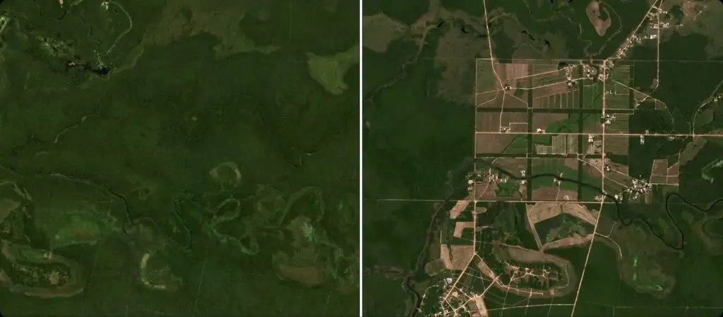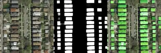

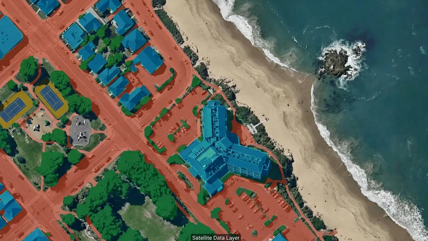
Describing a whole scene rather than detecting objects within it changes the nature of the work. Every pixel receives a class, no surface stays unanswered, and that exhaustiveness requires settling boundaries nobody would have had to decide in detection.
This article sets out those methods. It extends the satellite imagery guide.
What semantic segmentation produces
Four differences separate it from object detection in satellite imagery.
Every single pixel receives a class, with no exception and no empty zone.
Continuous surfaces count there as much as isolated objects.
No notion of instance comes to distinguish two objects of one class.
And the result obtained reads as a map rather than as a list.
One important practical consequence follows. The third difference directs the choice, counting buildings requiring instance segmentation where a built-up surface is satisfied by a single class.
The classes that structure a nomenclature
Six families of class occur in satellite imagery.
Built surfaces along with all artificialised spaces.
Agricultural surfaces, whether cultivated or under grass.
Forest environments along with the various wooded formations.
Water surfaces, whether permanent or temporary.
Bare soils along with the other mineral surfaces.
And linear infrastructure, traffic routes and networks.
One important observation follows for a satellite imagery project. The last family raises a difficulty of its own, a road being at once a surface and a linear object, which obliges deciding whether it belongs to the surface nomenclature or to separate handling.
What the boundary between classes requires
Five situations require an explicit convention in satellite imagery.
The edge between a forest and an immediately adjoining meadow.
The fringe separating an urban fabric from its agricultural periphery.
The bank, whose position varies with the level of the water itself.
A house’s garden, held to be built or vegetated depending on the viewpoint taken.
And the fallow field, agricultural or natural depending on how long it has lain.
One practical consequence follows. Those five situations recur on almost every tile, which makes their treatment more decisive for the corpus’s consistency than the choice of the classes themselves.
What granularity changes
Four satellite imagery effects accompany a detailed reference.
Annotation time grows far faster than the number of classes.
Confusions between neighbouring classes multiply rapidly.
Disagreement between annotators then rises very appreciably.
And some distinctions become quite simply impossible at the available resolution.
One important observation follows. The last effect bounds any ambition, a nomenclature distinguishing crops the pixel does not separate producing a corpus in which some classes stay undecidable whatever the care taken.
What exhaustive coverage imposes
Four constraints follow from the obligation to classify everything in satellite imagery.
No surface can be left without an explicit decision.
Ambiguous zones must still receive a class in spite of the doubt.
Clouds and cast shadows both require explicit treatment.
And the time spent per tile becomes predictable but high.
One important practical consequence follows for a satellite imagery project. The second constraint justifies a class of indetermination, failing which doubtful zones distribute themselves silently among the neighbouring classes according to each operator’s judgement.
What the tools bring
Five assistances occur in this satellite imagery work.
Automatic selection by similarity of colour or texture.
Propagating one class across a whole homogeneous zone.
Automatic filling of the surfaces left unclassified.
Superimposing an already existing cartographic layer.
And a pre-segmentation then corrected rather than produced.
One observation follows. The fourth assistance renders a considerable service and introduces a risk, an existing layer directing the tracing towards the state it describes rather than towards that of the image, which carries its own errors and its age forward into the new corpus.
What the season changes about classification
Five satellite imagery surfaces change appearance across the year.
A cultivated field, left bare in winter and covered in summer.
A broadleaf forest, whose canopy disappears during the cold season.
A wetland, whose extent varies very strongly from month to month.
A meadow, whose colour follows the rainfall very closely.
And a bare soil, which may be temporary or permanent as the case may be.
One important practical consequence follows for a satellite imagery project. The first surface requires a convention of date, a ploughed field having to be classified as agricultural rather than as bare soil, which presupposes reasoning on the land’s use and not on its appearance at the instant of capture.
What the measurement must reflect
Five indicators describe such a satellite imagery system’s performance.
The proportion of pixels correctly classified, all classes taken together.
Performance measured by class, which finally reveals the minority classes.
The quality of the boundaries traced, distinct from that of the surfaces.
Confusions examined by pairs rather than overall errors.
And the behaviour observed on territories absent from the training.
One important practical consequence follows. The first indicator misleads systematically in satellite imagery, a class covering most of the territory carrying the overall score on its own, which masks complete failure on the rare classes the project was nonetheless targeting.
What class imbalance imposes
Four effects accompany a very uneven distribution of classes.
The majority classes entirely dominate any overall measurement.
The rare classes appear very little in a random sample.
A control by sampling encounters them only rarely.
And enrichment of the corpus must target them explicitly.
One important observation follows for a satellite imagery project. The third effect makes the control misleading, a random rereading of tiles bearing almost entirely on the dominant classes, which requires a sampling directed at the classes the project is genuinely seeking to obtain.
What the corpus must cover here
Five axes structure a segmentation dataset in satellite imagery.
The types of landscape covered, from the heavily artificialised to the wholly natural.
The regions handled, whose forms and materials differ.
The seasons covered, which modify the appearance of several classes.
The transition zones, where all the ambiguous boundaries concentrate.
And the rare classes, systematically absent from an undirected sample.
One important observation follows. The fourth axis deserves a deliberate effort, transition zones being at once the most difficult and the least represented in a random selection, which produces a corpus rich in homogeneous surfaces and poor exactly where the system will fail.
What annotator disagreement reveals
Four satellite imagery insights come out of a double annotation on the same tiles.
The pairs of classes two operators do not separate in exactly the same way.
The proportion of surface on which they genuinely diverge.
The precise location of those divergences, almost always at boundaries.
And the classes whose definition remains understood differently.
One important practical consequence follows for a satellite imagery project. The third insight usefully directs the effort, a disagreement concentrated on narrow bands at a class edge indicating a problem of convention rather than of competence, which is corrected by a written rule and not by further training.
What a hierarchy of classes permits
Four satellite imagery benefits follow from a nomenclature organised in levels.
A coarse level stays applicable whenever the detail becomes undecidable.
Rare classes group together without any of the information being lost.
Performance can be measured at several levels of precision.
And one corpus serves several uses without having to be reworked.
One important observation follows for a satellite imagery project. The first benefit resolves the granularity problem elegantly, an annotator unable to distinguish two crops being able to retain the agricultural class of the level above, which produces accurate information rather than an invented distinction.
What consistency between tiles requires
Four satellite imagery defects appear at the junction of two neighbouring tiles.
One same surface classified differently either side of the tile boundary.
A class boundary that simply stops abruptly at the tile edge.
A linear object visibly offset from one tile to the next.
And a transition zone settled one way and then the other way.
One important practical consequence follows for a satellite imagery project. The first defect shows only after reassembly, a tile taken in isolation looking perfectly consistent, which requires a control on the reconstituted mosaic rather than on separate tiles.
What clouds and shadows impose
Four treatments occur for these disturbed surfaces in satellite imagery.
A wholly dedicated class, which explicitly isolates the unusable zones.
A mask applied before the annotation, which simply removes them from the work.
A classification of what can be guessed beneath the disturbance.
And the use of another acquisition date to fill the zone concerned.
One important practical consequence follows for a satellite imagery project. The third treatment looks generous and proves harmful, a surface classified from a supposition entering the corpus on the same footing as an observation, which teaches the system to guess rather than to signal the absence of information.
What this work’s throughput presupposes
Four factors determine the time spent on one satellite imagery tile.
The number of classes genuinely present in the scene.
The total length of the boundaries to be traced.
The proportion of ambiguous zones actually encountered.
And the fineness required in tracing the outlines.
One important observation follows for a satellite imagery project. The second factor explains a considerable gap between territories, a fragmented peri-urban area demanding several times the time of an agricultural plain of the same surface, which makes any per-tile costing misleading without an indication of the landscape type.
What comparison between dates requires here
Four conditions make two satellite imagery segmentations comparable.
A class nomenclature strictly identical between the two dates.
A perfectly exact superimposition of the underlying images.
Boundary conventions unchanged from one campaign to the next.
And an equivalent season for all the classes that depend on it.
One important practical consequence follows for a satellite imagery project. The third condition is the most fragile over time, an edge rule modified between two campaigns producing a forest advance or retreat that reflects no real change in the territory.
What the delivery format changes
Four forms of output occur for delivering satellite imagery segmentation.
A class image, where each pixel carries a class identifier.
Vector polygons, which describe every surface by its own outline.
A separate layer per class, superimposable in a geographic system.
And a mixed format, combining raster for surfaces and vector for objects.
One important observation follows. The second form is the most requested and the most expensive to produce, an automatic conversion from a mask producing jagged outlines that have to be simplified, an operation whose settings modify the surfaces measured.
What this work demands of the annotator
Five aptitudes condition quality in satellite imagery segmentation.
Patience on tracing work that is both long and repetitive.
Rigour in applying a given boundary rule.
The capacity to recognise a zone they do not know how to classify.
A correct reading of the textures characterising each of the classes.
And sustained attention on tiles that are sometimes barely contrasted.
One important practical consequence follows. The third aptitude is the most decisive here, exhaustive coverage obliging decisions everywhere, which turns every hesitation into an assigned class if the operator has no means of signalling that they do not know.
What the minimum mapping unit fixes
Four effects follow from a surface threshold below which nothing is classified.
Isolated objects smaller than the threshold disappear entirely from the result.
The number of polygons left to produce then falls sharply.
Consistency between operators improves markedly on the small elements.
And the corpus becomes comparable with an existing map using the same threshold.
One important observation follows for a satellite imagery project. The first effect must be accepted explicitly, a copse or a pond smaller than the threshold being attached to the surrounding class, which constitutes an accepted loss of information rather than an annotation error.
What the first batch must establish
Four results justify a satellite imagery trial batch before production.
An average time per tile, measured separately on each type of landscape.
The list of boundary situations the reference had not foreseen.
A disagreement rate between two operators working the same tiles.
And the proportion of the surface that proves genuinely undecidable.
One important practical consequence follows for a satellite imagery project. The second result is what makes the trial worthwhile, a dozen tiles sufficing to reveal the cases nobody had envisaged at scoping, while discovering them in production requires reworking everything already delivered.
What the provider brings here
Four contributions distinguish a segmentation engagement on satellite imagery.
A reference settling the boundaries before production rather than during it.
A control conducted on the reconstituted mosaic and not on isolated tiles.
A sampling deliberately directed at the rare classes and the transition zones.
And a disagreement measurement returned alongside the delivered corpus.
One important practical consequence follows. The second contribution attracts little notice and costs little, a control by junction revealing inconsistencies no rereading of tiles shows, which makes it the most worthwhile arrangement specific to this kind of project.
Approaching a segmentation project
Five questions scope such a project in satellite imagery.
Are instances or surfaces needed. That changes the method.
Are the ambiguous boundaries settled. They recur everywhere.
Is the granularity compatible with the resolution. Otherwise classes stay undecidable.
Does a class of indetermination exist. Without it the doubt dissolves.
And is the measurement broken down by class. The overall average misleads.
Those five answers determine the corpus’s consistency. Asking them before production avoids a nomenclature part of which will never be applied reproducibly.
The question that frames the nomenclature
One question determines the reference to adopt in satellite imagery.
Do the classes serve a decision or a description.
A decision, authorising a construction or triggering an inspection, is satisfied by a few clear-cut classes and tolerates a coarse grouping of the other surfaces.
A description, a land-use inventory or statistical monitoring, requires a complete nomenclature, consistent between regions and compatible with existing references.
That question belongs to the use and not to technique, it is asked before the first tile, and it separates a nomenclature of five classes from one that will hold several dozen.
Three decisions before producing
Three decisions commit a segmentation project in satellite imagery.
Fixing a nomenclature whose every distinction stays decidable at the available resolution.
Writing the boundary rules for the five situations that recur everywhere.
And providing a class of indetermination, without which doubt dissolves silently.
Those three decisions cost one meeting, they precede the first tile, and their absence produces a nomenclature part of which will never be applied reproducibly.
Three checks on a segmented corpus
Three checks qualify a segmentation dataset in satellite imagery.
Performance broken down by class rather than an overall proportion of pixels.
The written rule for boundaries between neighbouring classes.
And the presence of transition zones within the annotated tiles.
Those three checks are each asked in one question, they require no cartographic competence, and their absence indicates a corpus whose announced score reflects above all the most extensive class.
What this chapter teaches
One cross-cutting observation deserves closing this examination.
Exhaustiveness obliges settling what detection permitted ignoring.
Three findings compose it.
Boundaries between neighbouring classes recur on almost every tile.
An overall measurement of correctly classified pixels masks failure on the rare classes.
And a granularity incompatible with the resolution produces undecidable classes.
That finding extends the preceding chapter, describing a whole scene requiring more conventions than detecting isolated objects.
What this chapter leaves to the next
A built-up surface says nothing of the number of buildings it holds.
Three questions stay open in satellite imagery.
How to separate adjoining constructions into distinct objects.
What a building’s exact footprint presupposes as a convention.
And how to handle the offset between visible roof and ground base.
Those three questions belong to building detection, which constitutes the subject of the following chapter.
Why per-tile pricing needs a caveat
One clarification belongs in any quotation for this work.
A tile is not a unit of work, only a unit of surface.
Three reasons follow in satellite imagery.
Boundary length varies by an order of magnitude between landscapes.
A fragmented peri-urban tile holds many times the work of a farmland one.
And the class count present drives the time as much as the area does.
One important practical consequence follows for a satellite imagery provider. Stating this at quotation stage protects both sides, since a rate agreed on farmland tiles and then applied to urban ones ends in a renegotiation nobody wanted, while a rate banded by landscape type holds for the life of the project.
Common mistakes
These failures recur often enough that naming them is usually enough to avoid them.
- Measuring performance as an overall proportion of correct pixels.
- Adopting a granularity the resolution does not permit.
- Leaving boundaries between neighbouring classes to each person’s judgement.
- Omitting a class for the indeterminate zones.
- Controlling by random sampling despite a strong imbalance.
- Using an existing cartographic layer without checking its date.
- Handling clouds and shadows with no explicit convention.
- Confusing semantic segmentation with instance segmentation.
- Neglecting the quality of boundaries in favour of that of surfaces.
- Adding classes without measuring the disagreement they introduce.
What to take away
Semantic segmentation requires deciding what detection permitted setting aside.
Three readings emerge. Boundaries between neighbouring classes, woodland edges and peri-urban fringes, recur on almost every tile, which makes their treatment more decisive for the corpus’s consistency than the choice of the classes themselves. An overall measurement of correctly classified pixels misleads systematically, a class covering most of the territory carrying the score on its own and masking complete failure on the rare classes the project was targeting. And a granularity incompatible with the available resolution produces undecidable classes, a reference distinguishing crops the pixel does not separate staying inapplicable whatever the annotators’ care.
For footprint detection, the article on buildings and urban footprints details the approach. For the quality of the work, the article on small objects and visual fatigue sets it out.
To explore delivery arrangements, supported formats and applicable control mechanisms, see our dedicated page on annotation for geospatial. And if you are preparing a segmentation project, let us discuss your need.